Regression

Assume that we have dataset \(\mathcal{D}={(\mathbf{x}_1, y_1,...,(\mathbf{x}_n,y_n)}\) where \(\mathbf{x}_i\in\mathbb{R}^m\) and \(y_i\in\mathbb{R}\), where \(\mathbf{x}_i\) consists of \(m\) measurements or attributes associated with the \(i\)-th observation and \(y_i\) is the \(i\)-th target variable which is some real number. Then we are interested in learning some functional map that maps from our observation space to our target space i.e. \(\mathcal{X}\rightarrow\mathcal{Y}\). There are a multitude of assumptions we could make about defining the best \(f\) but the most popular is to assume \(f\) is the curve of best fit through our data and the noise present is Gaussian. Mathematically we can define the functional relationship to be

\[\begin{equation} y_i = f(\mathbf{x}_i;\boldsymbol{\theta}) + \epsilon_i, \qquad \epsilon_i \overset{\text{iid}}{\sim}\mathcal{N}(0,\sigma^2), \end{equation}\]

where \(\boldsymbol{\theta}\) are the parameters for our functional map \(f\) and \(\epsilon_i\) is some random Gaussian noise. The reason why we can assume that noise is present is because we often may not have all the information in \(\mathbf{X}\) to construct \(\mathbf{y}\) or our proposed function \(f\) may be simpler than the true function \(f^{*}\) and so we are finding the best simpler model that fits the more complicated dataset.

From Eq. (1), we can say that our predictor for \(y_i\) is \(\mathbb{E}[f(\mathbf{x}_i;\boldsymbol{\theta}) + \epsilon_i] = \mathbb{E}[f(\mathbf{x}_i;\boldsymbol{\theta})]\). For notational convenience let us denote \(\mu(\mathbf{x}_i;\boldsymbol{\theta}) = \mathbb{E}[f(\mathbf{x}_i;\boldsymbol{\theta})]\), and assume that our function \(f\) is deterministic i.e. a strict one to one map. We can then say that

\[\begin{equation} y_i|\mathbf{x}_i,\boldsymbol{\theta},\sigma^2 \overset{\text{iid}}{\sim}\mathcal{N}(\mu(\mathbf{x}_i; \boldsymbol{\theta}),\sigma^2), \end{equation}\]

that is, our target variable given an associated distribution follows an independent and identically distributed Gaussian with mean \(\mu(\mathbf{x}_i,\boldsymbol{\theta})\) and variance \(\sigma^2\). To visualise the relationships between the variables we have the below.

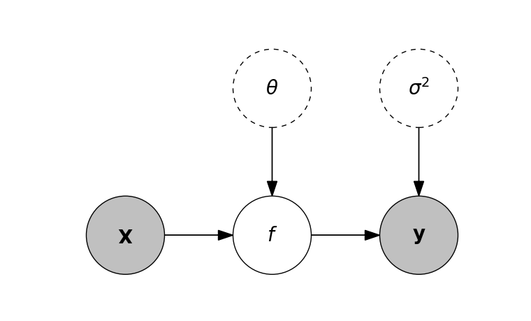
Fig. 39 Graphical model representation of the regression problem. Dotted circles are the unknowns of interest, shaded circles are the data, and regular circles are functions.

Writing the conditional probability density of Eq. (2) we yield

\[\begin{equation} p(y_i|\mathbf{x}_i,\boldsymbol{\theta},\sigma^2) = (2\pi\sigma^2)^{-\frac{1}{2}}\exp\bigg(-\frac{1}{2\sigma^2}\big(y_i - \mu(\mathbf{x}_i;\boldsymbol{\theta})\big)^2\bigg). \label{eq:normal-pdf} \end{equation}\]

Assuming that each of the \(n\) observations are independent, we can state

\begin{align} p(\mathbf{y}|\mathbf{X},\boldsymbol{\theta},\sigma^2) &= \prod_{i=1}^n p(y_i|\mathbf{x}_i,\boldsymbol{\theta},\sigma^2), \label{eq:likelihood}\\ &= (2\pi\sigma^2)^{-\frac{n}{2}}\exp\bigg(-\frac{1}{2\sigma^2}\sum_{i=1}^n\big(y_i - \mu(\mathbf{x}_i;\boldsymbol{\theta})\big)^2\bigg), \\ \log p(\mathbf{y}|\mathbf{X},\boldsymbol{\theta},\sigma^2) &= -\frac{n}{2}\log 2\pi\sigma^2 - \frac{1}{2\sigma^2}\sum_{i=1}^n\big(y_i - \mu(\mathbf{x}_i;\boldsymbol{\theta})\big)^2, \label{eq:sum}\\ &= -\frac{n}{2}\log 2\pi\sigma^2 - \frac{1}{2\sigma^2}\big(\mathbf{y} - \boldsymbol{\mu}(\mathbf{X};\boldsymbol{\theta})\big)^\text{T}\big(\mathbf{y} - \boldsymbol{\mu}(\mathbf{X};\boldsymbol{\theta})\big), \label{eq:transpose}\\ &= -\frac{n}{2}\log 2\pi\sigma^2 - \frac{1}{2\sigma^2}||\mathbf{y} - \boldsymbol{\mu}(\mathbf{X};\boldsymbol{\theta})||_2^2. \label{eq:norm} \end{align}

Note

The notation used in Eqs. (6-8) all mean the same thing.

For simplicity, let \(\mathbf{z} = \mathbf{y} - \boldsymbol{\mu}(\mathbf{X};\boldsymbol{\theta})\) and to simplify further assume that \(\mathbf{z}\in\mathbb{R}^{3}\) i.e. \(\mathbf{z} = [z_1,z_2,z_3]\), then:

\begin{align*} \mathbf{z}^\text{T}\mathbf{z} &= \begin{bmatrix} z_1 & z_2 & z_3\end{bmatrix} \begin{bmatrix}z_1\\z_2\\z_3\end{bmatrix},\\ &= z_1^2 + z_2^2 + z_3^2, \\ &= \sum_{i = 1}^3 z_i^2. \end{align*}

The jump from Eq. \(\eqref{eq:sum}\) to Eq. \(\eqref{eq:transpose}\) is now explained. Eq. \(\eqref{eq:norm}\) comes from the definition of a vector norm.

\begin{align*} ||\mathbf{z}||_p^q :&= \bigg[\sum_{i = 1}^3 |z_i|^p\bigg]^{q / p}, \\ ||\mathbf{z}||_2^2 &= \bigg[\sum_{i=1}^3 |z_i|^2\bigg]^{2 / 2} (\text{setting } p = q = 2),\\ &= \sum_{i=1}^3 z_i^2. \end{align*}

The probability distribution \(p(\mathbf{y}_i\mid\mathbf{x}_i,\boldsymbol{\theta},\sigma^2)\) stated in Eq. \(\eqref{eq:normal-pdf}\) indicates a distribution over \(\mathcal{Y}\) with the most probable value to be \(\mu(\mathbf{x}_i;\boldsymbol{\theta})\). Likewise, for the entire dataset, the most likely set of values associated with \(\mathbf{X}\) is \(\boldsymbol{\mu}(\mathbf{X},\boldsymbol{\theta})\). In plain english, the left hand side of Eq. \(\eqref{eq:likelihood}\) is the likelihood (or probability) that we would observe \(\mathbf{y}\) if we started from \(\mathbf{X}\) and used Eq. (1) to generate \(\mathbf{y}\). If the probability is low then we have a poor functional map \(f\) and similarly, if we the probability is high then we have a good functional map \(f\). As the function log just converts the probability space \((0,1)\) to the log probability space \((-\infty,0)\), we can choose to maximise the log probability instead. This is often done in practice as the resulting math is much easier and maximising the log probability also maximises the probability.

To maximise Eqs. (\(\ref{eq:sum}\)-\(\ref{eq:norm}\)) (all the same expression) with respect to \(\boldsymbol{\theta}\), we can consider all other variables constants and simply ignore them for the optimisation step. We can see that maximising the log probability is equivalent to minimising

\[\begin{equation} \mathcal{L}(\boldsymbol{\theta};\mathbf{X},\mathbf{y}) := ||\mathbf{y} - \boldsymbol{\mu}(\mathbf{X};\boldsymbol{\theta})||_2^2. \end{equation}\]

To minimise \(\mathcal{L}(\boldsymbol{\theta};\mathbf{X},\mathbf{y})\), we can consider the Jacobian (first derivative) and perform gradient descent,

\[\begin{equation} \nabla_{\boldsymbol{\theta}} \mathcal{L}(\boldsymbol{\theta};\mathbf{X},\mathbf{y}) = -2\nabla_{\boldsymbol{\theta}} [\boldsymbol{\mu}(\mathbf{X};\boldsymbol{\theta})]^\text{T}\odot\big(\mathbf{y} - \boldsymbol{\mu}(\mathbf{X};\boldsymbol{\theta})\big), \label{eq:grad} \end{equation}\]

where \(\odot\) denotes element-wise multiplication.

Note

Differentiating the loss function.

\(\nabla_\theta \mathcal{L}(\theta;\mathbf{X},\mathbf{y})\) means the vector differential of \(\mathcal{L}(\theta;\mathbf{X},\mathbf{y})\) with respect to \(\theta\). Suppose that there are three parameters \(\theta_1,\ \theta_2 \text{ and } \theta_3\), and we want to find the differential of \(\mathcal{L}((\theta_1, \theta_2, \theta_3);\mathbf{z}) = ||\mathbf{z}(\theta_1,\theta_2,\theta_3)||_2^2\) with respect to \(\theta_1\) where \(\mathbf{z} = [z_1,z_2,z_3]\) then:

\begin{align*} \frac{\partial \mathcal{L}}{\partial \theta_1} &= \frac{\partial}{\partial \theta_1}\bigg[||\mathbf{z}||_2^2\bigg],\\ &= \frac{\partial}{\partial \theta_1}\bigg[\sum_{i=1}^3 z_i^2\bigg], \\ &= \sum_{i=1}^3 \frac{\partial}{\partial \theta_1} [z_i^2], \\ &= \sum_{i=1}^3 2\frac{\partial}{\partial \theta_1}[z_i] z_i,\\ &= 2\frac{\partial \mathbf{z}}{\partial \theta_1}^\text{T}\mathbf{z},\\ \Rightarrow \nabla_{\theta} [\mathcal{L}] &= \begin{bmatrix}\frac{\partial \mathcal{L}}{\partial \theta_1} \\ \frac{\partial \mathcal{L}}{\partial \theta_2} \\ \frac{\partial \mathcal{L}}{\partial \theta_3}\end{bmatrix},\\ &= 2\begin{bmatrix}\frac{\partial \mathbf{z}^\text{T}}{\theta_1}\mathbf{z} \\ \frac{\partial \mathbf{z}^\text{T}}{\theta_2}\mathbf{z} \\ \frac{\partial \mathbf{z}^\text{T}}{\theta_3}\mathbf{z}\end{bmatrix}, \\ &= 2\nabla_{\theta} [\mathbf{z}]^\text{T} \odot \mathbf{z}, \end{align*}

where \(\odot\) denotes element-wise multiplication.

If our functional map \(f\) is linear, we can solve Eq. \(\eqref{eq:grad}\) directly and this is called linear regression, if it is non-linear, we typically cannot solve it and have to resort to gradient descent. For all deterministic functional maps \(f\), this underlying theory will apply. If the functional map \(f\) is stochastic i.e. has an underlying distribution a more general set of assumptions will have to be made around the variance \(\sigma^2\) attributed to the distribution of \(\mathbf{y}\) as there will be covariances introduced. See the gaussian process as an example.