Gaussian Process Regression
Building on the Bayesian Linear Regression framework, we had to initially choose a couple of things:
How many basis functions should we use?
Where should the \(\mathbf{C}\) locations be positioned?
The Gaussian Process (GP) answers these two problems for us!
Recall that the general regression framework is that for a dataset \(\mathcal{D}=\{(\mathbf{x}_1,y_1),...,(\mathbf{x}_n,y_n)\}\) we want to find
What do we want our \(f\) function to look like and are there any properties we desire? Lets make only one assumption - the function \(f\) is smooth and we would like some error bars! If we want smoothness, we can say that if \(\mathbf{x}_1\) and \(\mathbf{x}_2\) are similar then the associated target values \(y_1\) and \(y_2\) are also similar. To help encode this we can consider a function of the norm of the difference \(||\mathbf{x}_1-\mathbf{x}_2||\) (see A2). If we did consider this as how correlated points were, it would have the adverse effect as the norm goes to 0 when the difference goes to 0. To ensure that when the difference is small, there is high correlation, we can take the exponent of this norm. We can express this two data point example as
where \(g\) is a function that we can choose. We can now encode a prior on continuous functions. One popular choice of the covariance kernel is the squared-exponential kernel (also known as the Gaussian or Radial Basis Function kernel) defined as
where \(\sigma_s^2\) and \(l\) are the signal variance and lengthscale of the kernel respectively. The lengthscale modulates the relationship between the smoothness and the distance between the \(x\) locations. Other popular choices of kernels can be found on Kernel Cookbook or Wikipedia.
The joint distribution between the observed dataset and a new datapoint can be now written as
where \(m\) is a mean function, \(\mathbf{x}^{*}\) is a new observation and \(y^{*}\) is the associated target variable. The choice of mean function is up to the user but can be as simple as the mean value of \(\mathbf{y}\) to another model e.g. a Linear Regression model. We can solve for the posterior estimate of \(y^{*}\) in closed form yielding
Note
Derivation of the (noise-free) predictive posterior
where
which implies
Substituting into \(\eqref{star}\) yields
In practice we have \(y = f(\mathbf{x}) + \epsilon\) with \(\epsilon\overset{\text{iid}}{\sim}\mathcal{N}(0,\sigma^2)\) so we can encorporate this independent noise yielding
From the above we have a means of computing predictions (and quantify the uncertainty around them). By considering the first block elements in the joint distribution as defined in Eq. \(\eqref{eq:joint}\) we have
which is also referred to as \(\mathcal{GP}(\mathbf{m},\mathbf{K} + \sigma^2\mathbf{I})\) in the literature. Expressing the above in log probabilities we have
where we introduce \(\theta\) to be the parameters of the covariance kernel. Examining the three terms from left to right, we have the normalisation constant which can be ignored from an optimisation point of view, the log determinant which measures model complexity, and finally the quadratic term which measures data fit. The GP naturally has this in-built regularisation term which penalises the model if it gets to complicated (which reduces the chance of our model overfitting). If \(\theta\) is constrained to positive values (such as the squared exponential kernel and many other kernels) then we need to ensure it never becomes negative. One simple trick to do that is to optimise the parameters in log space as when we exponentiate our logarithmic values we are strictly positive.
Let \(\mathbf{V} = k(\mathbf{X},\mathbf{X};\theta) + \sigma^2\mathbf{I}\) then partially differentiating the log probability yields
Example: Load Boston
Dataset
load_boston
Data Set Characteristics:
- Number of Instances
506
- Number of Attributes
13 numeric/categorical predictive. Median Value (attribute 14) is usually the target.
- Attribute Information (in order)
CRIM per capita crime rate by town
ZN proportion of residential land zoned for lots over 25,000 sq.ft.
INDUS proportion of non-retail business acres per town
CHAS Charles River dummy variable (= 1 if tract bounds river; 0 otherwise)
NOX nitric oxides concentration (parts per 10 million)
RM average number of rooms per dwelling
AGE proportion of owner-occupied units built prior to 1940
DIS weighted distances to five Boston employment centres
RAD index of accessibility to radial highways
TAX full-value property-tax rate per $10,000
PTRATIO pupil-teacher ratio by town
B 1000(Bk - 0.63)^2 where Bk is the proportion of blacks by town
LSTAT % lower status of the population
MEDV Median value of owner-occupied homes in $1000’s
- Missing Attribute Values
None
- Creator
Harrison, D. and Rubinfeld, D.L.
This is a copy of UCI ML housing dataset. https://archive.ics.uci.edu/ml/machine-learning-databases/housing/
This dataset was taken from the StatLib library which is maintained at Carnegie Mellon University.
The Boston house-price data of Harrison, D. and Rubinfeld, D.L. ‘Hedonic prices and the demand for clean air’, J. Environ. Economics & Management, vol.5, 81-102, 1978. Used in Belsley, Kuh & Welsch, ‘Regression diagnostics …’, Wiley, 1980. N.B. Various transformations are used in the table on pages 244-261 of the latter.
The Boston house-price data has been used in many machine learning papers that address regression problems.
Belsley, Kuh & Welsch, ‘Regression diagnostics: Identifying Influential Data and Sources of Collinearity’, Wiley, 1980. 244-261.
Quinlan,R. (1993). Combining Instance-Based and Model-Based Learning. In Proceedings on the Tenth International Conference of Machine Learning, 236-243, University of Massachusetts, Amherst. Morgan Kaufmann.
Python
Define kernel and kernel gradients
from   sklearn.datasets import load_boston
from   matplotlib       import pyplot as plt
import numpy as np

def squared_exponential(X1, X2, l, s2):
    return s2 * np.exp(-cdist(X1, X2, 'sqeuclidean') / (2 * np.square(l)))

def squared_exponential_gradient(X1, X2, l, s2):
    D = cdist(X1, X2, 'sqeuclidean')
    K = s2 * np.exp(-cdist(X1, X2, 'sqeuclidean') / (2 * np.square(l)))
    return [D * K, K]

def rational_quadratic(X1, X2, l, a, s2):
    return s2 * (1 + cdist(X1, X2, 'sqeuclidean') / (2 * a * np.square(l))) ** -a

def rational_quadratic_gradient(X1, X2, l, a, s2):
    D    = cdist(X1, X2, 'sqeuclidean')
    D2al = D / (2 * a * np.square(l))
    f    = 1 + D2al
    k    = s2 * f ** -(a + 1)
    K    = s2 * f ** -(a)
    return [s2 * 2 * D2al * k, D2al * K * np.log(f), K]
Gaussian Process Class
1 2 3 4 5 6 7 8 9 10 11 12 13 14 15 16 17 18 19 20 21 22 23 24 25 26 27 28 29 30 31 32 33 34 35 36 37 38 39 40 41 42 43 44 45 46 47 48 49 50 51 52 53 54 55 56 57 58 59 60 61 62 63 64 65 66 67 68 69 70 71 72 73 74 75 76 77 78 79 80 81 82 83 84 85 86 87 88 89 90 | class GaussianProcess():
"""
Gaussian Process Class
Parameters
====================
kernel : function
Covariance kernel function.
kernel_gradient : function
Computes the partial derivatives of the kernel function w.r.t. the parameters in the order they are used.
mean_function : function
Mean function for the Gaussian Process framework.
random_state : int
Parameter to be used in numpy.random.seed for reproducible results.
"""
def __init__(self, kernel, kernel_gradient, mean_function = None, random_state = None):
self.K = kernel
self.Kg = kernel_gradient
self.m = mean_function
self._params = dict(random_state = random_state)
def fit(self, X, y, alpha = 0.1, momentum = 0.1, epochs = 150):
n, m = X.shape
# Generate mean function if None provided
if self.m is None:
self.m = lambda X : np.ones((len(X), 1)) * y.mean()
# Shift and rescale targets
y = (y - self.m(X))
scale = self.scale = y.std()
y /= scale
# Scale alpha
alpha /= n
np.random.seed(self._params['random_state'])
# Ignore X1 and X2 but include an additional noise variance parameter
nparams = self.K.__code__.co_argcount - 2 + 1
# Initialise the log parameters and their gradients
lparams = self.lparams = np.random.normal(scale = 0.5, size = nparams)
gparams = np.zeros(nparams)
const = n / 2 * np.log(2 * np.pi)
# Store each component of the negative loss likelihood
loss = self.loss = np.zeros((epochs + 1, 3))
for i in range(epochs):
K = self.K(X, X, *np.exp(lparams[:-1]))
V = K + np.eye(n) * np.exp(lparams[-1])
Ki = np.linalg.inv(V)
Kiy = Ki @ y
loss[i] = const, np.linalg.slogdet(V)[1], y.T @ Kiy
# Update parameters (with momentum)
for j, grad in enumerate(self.Kg(X, X, *np.exp(lparams[:-1]))):
gparams[j] *= momentum
gparams[j] += (np.trace(Kiy.T @ grad @ Kiy) - np.trace(Ki @ grad))
lparams[j] += alpha * gparams[j]
gparams[-1] *= momentum
gparams[-1] += np.exp(lparams[-1]) * (np.trace(Kiy.T @ Kiy) - np.trace(Ki))
lparams[-1] += alpha * gparams[-1]
K = self.K(X, X, *np.exp(lparams[:-1]))
V = K + np.eye(n) * np.exp(lparams[-1])
Ki = self.Ki = np.linalg.inv(V)
Kiy = self.Kiy = Ki @ y
loss[-1] = const, np.linalg.slogdet(V)[1], y.T @ Kiy
loss /= n
self.k = lambda z : self.K(z, X, *np.exp(lparams[:-1]))
return self
def __call__(self, X, var = False):
mu = self.k(X) @ self.Kiy * self.scale + self.m(X)
if var:
Kxx = self.K(X, X, *np.exp(self.lparams[:-1]))
KxX = self.k(X)
cov = Kxx + KxX @ self.Ki @ KxX.T
var = np.diag(cov)
return mu, var
return mu
|
Load the data and create linear model and rmse function
X, y = load_boston(return_X_y = True)
y.resize(len(y), 1)

X_train, X_test, y_train, y_test = train_test_split(X, y, random_state = 2021)

w = np.linalg.lstsq(np.insert(X_train, 0, 1, 1), y_train, rcond = -1)[0]

def linear(X):
    return np.insert(X, 0, 1, 1) @ w

def rmse(model, X, y):
    return np.sqrt(np.mean(np.square(model(X) - y)))
Model training and evaluation
model1 = GaussianProcess(squared_exponential, squared_exponential_gradient, mean_function = linear, random_state = 2021).fit(X_train, y_train)
model2 = GaussianProcess(rational_quadratic , rational_quadratic_gradient , mean_function = linear, random_state = 2021).fit(X_train, y_train)

# Test the trained model with both kernels against the linear case to see if there is any improvement beyond the linear model
[rmse(model, X_test, y_test) for model in (linear, model1, model2)]
# [4.758342005376841, 4.7583318332395335, 4.647409609017597]
It seems that both kernels could learn beyond the linear regression mean function (with the squared exponential kernel barely doing so). Visualising the loss over training iterations we have the following plots.
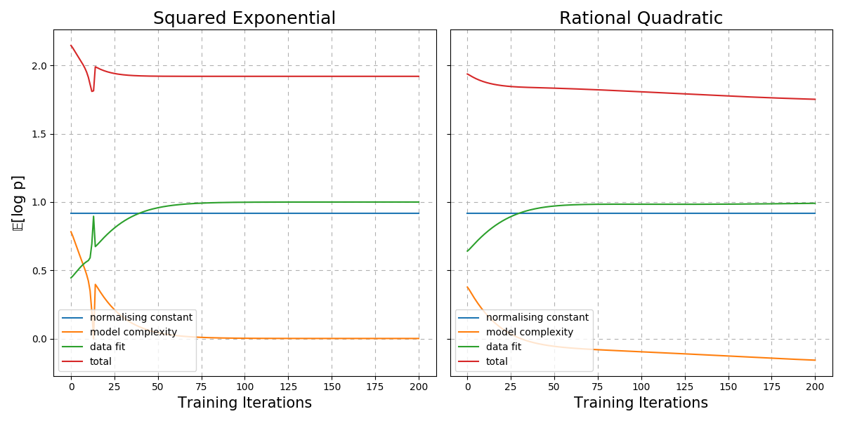
Fig. 30 Comparison of the expected negative log likelihood of the Gaussian process with the squared exponential and rational quadratic kernels.
By comparison, it seems the rational quadratic kernel is slightly more suited to this dataset as the total log probability is lower (and continuing to decrease). Lets try to visualise the error bars on a toy problem.
Example: Noisy sin function
Python
Data generator
def generator(n, m, func, domain = (0, np.pi * 2), scale = 0.15, random_state = None):
    """
    Data Generator

    Parameters
    =================
        n            : int
                       Number of training samples to generate.

        m            : int
                       Number of dimensions each observation has.

        func         : function
                       True function to learn.

        domain       : list, tuple
                       Domain for each dimension of our observations defining the interval [a, b].

        scale        : float
                       The standard deviation parameter for the additive Gaussian noise.

        random_state : int
                       Parameter to be used in numpy.random.seed for reproducible results.
    """
    # Set seed for X
    np.random.seed(random_state)

    # Training data
    xjs = [np.random.uniform(*domain, size = n) for _ in range(m)]
    X   = np.array([xj.flatten() for xj in np.meshgrid(*xjs)]).T
    t   = func(X)

    # Set seed for y
    np.random.seed(random_state)

    y   = t + np.random.normal(scale = scale, size = t.shape)

    # True function (at x10 resolution and 10% outside domain)
    d   = domain[0] - (domain[1] - domain[0]) * 0.1, domain[1] + (domain[1] - domain[0]) * 0.1
    xj  = [np.linspace(*d, 11 * n) for _ in range(m)]
    x   = np.array([x.flatten() for x in np.meshgrid(*xj)]).T
    t   = func(x)

    return X, y, x, t
Generating a training on 10 noisy sin data points
X, y, x, t = generator(10, 1, np.sin, random_state = 2021)

model1 = GaussianProcess(squared_exponential, squared_exponential_gradient, random_state = 2021).fit(X, y, alpha = 0.1, momentum = 0.8)
model2 = GaussianProcess(rational_quadratic , rational_quadratic_gradient , random_state = 2021).fit(X, y, alpha = 0.1, momentum = 0.8)

fig, ax = plt.subplots(1, 2, figsize = (12, 4), sharey = True)

for i, (model, title) in enumerate(zip([model1, model2], ['Squared Exponential', 'Rational Quadratic'])):

    ax[i].plot(x, t, color = cmap.colors[0])
    ax[i].scatter(X, y, color = 'k', zorder= 3)

    mu, var = model(x, var = True)
    std     = np.sqrt(var)

    ax[i].plot(x, mu, color = cmap.colors[1])
    ax[i].fill_between(x.flatten(), mu.flatten() + 2 * std, mu.flatten() - 2 * std, color = cmap.colors[1], alpha = 0.5)
    ax[i].grid(ls = (0, (5, 5)))
    ax[i].set_title(title)

    ax[i].set_xticks(np.arange(0, 2.1, 0.5) * np.pi)
    ax[i].set_xticklabels(['$0$', r'$\rm\pi/2$', r'$\rm\pi$', r'$\rm3\pi/2$', r'$\rm2\pi$'])
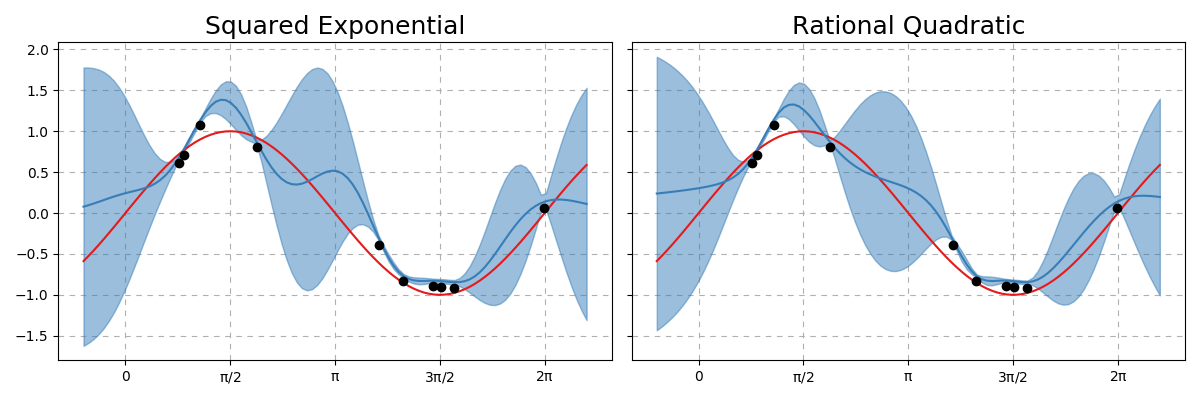
Fig. 31 Comparison of Gaussian Process kernels on 10 noisy sin data points. Blue line is the mean with the shaded region within 2 standard deviations away from the mean.
It seems that when there is little data around, the uncertainty of our model increases! This makes intuitive sense as we are less sure about computing inference at an unfamiliar \(x^{*}\) location. Both kernels seem to perform similarly. Lets see how that changes as we increase the number of samples from 10 to 50.
Python
Generating a training on 50 noisy sin data points
X, y, x, t = generator(50, 1, np.sin, random_state = 2021)

model1 = GaussianProcess(squared_exponential, squared_exponential_gradient, random_state = 2021).fit(X, y, alpha = 0.1, momentum = 0.8)
model2 = GaussianProcess(rational_quadratic , rational_quadratic_gradient , random_state = 2021).fit(X, y, alpha = 0.1, momentum = 0.8)

fig, ax = plt.subplots(1, 2, figsize = (12, 4), sharey = True)

for i, (model, title) in enumerate(zip([model1, model2], ['Squared Exponential', 'Rational Quadratic'])):

    ax[i].plot(x, t, color = cmap.colors[0])
    ax[i].scatter(X, y, color = 'k', zorder= 3)

    mu, var = model(x, var = True)
    std     = np.sqrt(var)

    ax[i].plot(x, mu, color = cmap.colors[1])
    ax[i].fill_between(x.flatten(), mu.flatten() + 2 * std, mu.flatten() - 2 * std, color = cmap.colors[1], alpha = 0.5)
    ax[i].grid(ls = (0, (5, 5)))
    ax[i].set_title(title)

    ax[i].set_xticks(np.arange(0, 2.1, 0.5) * np.pi)
    ax[i].set_xticklabels(['$0$', r'$\rm\pi/2$', r'$\rm\pi$', r'$\rm3\pi/2$', r'$\rm2\pi$'])
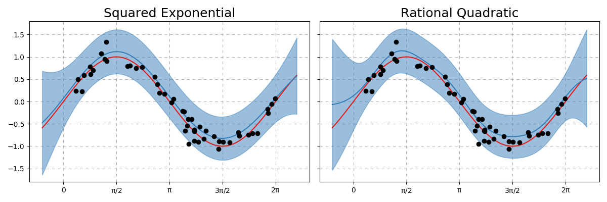
Fig. 32 Comparison of Gaussian Process kernels on 50 noisy sin data points. Blue line is the mean with the shaded region within 2 standard deviations away from the mean.
From the above, we can see that the uncertainty quantification is much more smooth and generally follows that of a sin function. Where we do not have any data (the far left and right regions) the uncertainty quantification increases significantly with the mean to have the tendancy to curve towards 0 (as this was assumed to be the mean function). Additionally, it seems like the rational quadratic kernel was not right for this problem as the general shape is less sin like compared to the squared exponential kernel.
Hint
A periodic kernel would have been the best kernel for this problem.