Logistic Regression

Building upon the theory of classification , in what follows, we assume that we have a supervised dataset \(\mathcal{D} = \{(\mathbf{x}_1,\mathbf{y}_1),...,(\mathbf{x}_n,\mathbf{y}_n)\}\) where \(\mathbf{x}_i\in\mathbb{R}^{m}\) is a set of \(m\) real valued measurements or features for the \(i\)-th observation, and \(\mathbf{y}_i\in\{0,1\}^c\) indicates which of the \(c\) classes the \(i\)-th observation attributes to.

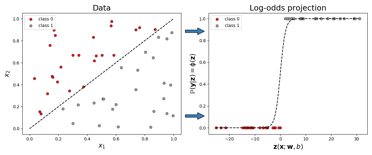
Fig. 5 Example illustration of Logistic Regression.

Example simulated data for (binary) logistic regression. On the left, we have our dataset with a clear linear boundary separating the two classes. The right is a linear transform which separates the two classes about the origin and quantifies the probability of belonging to class 1.

In the case of binary classification i.e. only two classes, the objective of logistic regression is very clear from the above plots; We wish to find the equation of the linear boundary separating the two classes. When the data is more than 2D then we wish to find the boundary hyperplane. For binary logistic regression \(\mathbf{z} := \mathbf{Xw} + b\) and so the gradients of the two parameters are given by \(\nabla_{\mathbf{w}} \mathbf{z} = \mathbf{X}\) and \(\nabla_{b} \mathbf{z} = \mathbb{1}\). Plugging both into Eq. (14) in classification#binary-classification , we yield

\begin{align} \mathbf{g}_{t + 1} &\leftarrow \mathbf{y} - \hat{\mathbf{y}}, \\ \mathbf{w}_{t + 1} &\leftarrow \mathbf{w}_t + \alpha \mathbf{X}^\text{T}\mathbf{g}_{t+1}, \label{eq:w}\\ b_{t+1} &\leftarrow b_t + \alpha \mathbf{1}^\text{T}\mathbf{g}_{t + 1}, \label{eq:b} \end{align}

where \(\alpha > 0\) is referred to as the step-size or learning rate, and \(\mathbf{\hat{y}}_t := \phi(\mathbf{Xw}_t + b_t)\).

Python

Logistic Regression class

from   sklearn.model_selection import train_test_split
from   sklearn                 import datasets as ds
import numpy as np

class LogisticRegression():
    """
    Logistic Regression class

    Parameters
    =================
        loss         : function
                       Loss function to be evaluated at every time step.

        phi          : function
                       Function to map the log-odds to probability space.

        momentum     : float
                       Momentum for the gradient optimisation (speeds up convergence).

        random_state : int
                       Parameter to be used in numpy.random.seed for reproducible results
    """
    def __init__(self, loss, phi, momentum = 0.99, random_state = None):
        self.loss         = loss
        self.phi          = phi
        self.momentum     = momentum
        self.random_state = random_state

    def fit(self, X, Y, X_val = None, Y_val = None, alpha = 1e-6, epochs = 2000):

        np.random.seed(self.random_state)

        # Detect if validation data has been given
        v = isinstance(X_val, np.ndarray)

        # Initialise W and b
        # Common to initialise W randomly and b at zero
        m = X.shape[1]
        c = 1 if Y.ndim == 1 else Y.shape[1]

        if c == 1:
            W = self.W = np.random.normal(scale = 0.01, size = m)
            b = self.b = 0
        else:
            W = self.W = np.random.normal(scale = 0.01, size = (m, c))
            b = self.b = np.zeros(c)

        if v:
            # Store all of the validation "Z" values
            Zs = []

        # Loss (and validation loss if provided)
        L    = np.zeros((epochs + 1, 1 + v))

        # Initialise gradients for W and b to be 0
        gW   = 0
        gb   = 0
        for i in range(epochs):
            hat  = self.phi(X @ W + b)
            L[i] = self.loss(Y, hat)
            if v:
                Zs.append(X_val @ W + b)
                L[i, 1] = self.loss(Y_val, self.phi(Zs[-1]))
            hat  = self.phi(X @ W + b)
            g    = (Y - hat) / len(Yb)
            gW  *= self.momentum
            gb  *= self.momentum
            gW  += X.T @ g          # Eq. (2)
            gb  += g.sum(axis = 0)  # Eq. (3)
            W   += alpha * gW
            b   += alpha * gb
        hat   = self.phi(X @ W + b)
        L[-1] = self.loss(Y, hat)
        if v:
            Zs.append(X_val @ W + b)
            L[-1, 1] = self.loss(Y_val, self.phi(Zs[-1]))
            Zs       = np.array(Zs)

        # Store the loss over time
        self.logs = dict(L = L)

        if v:
            # Store the validation "Z" values over time
            self.logs['Zs'] = Zs

        return self

    def __call__(self, X):
        return self.phi(X @ self.W + self.b)

Python

Sigmoid and binary cross entropy loss functions

def sigmoid(z):
    """ Logistic sigmoid function """
    return 1 / (1 + np.exp(-z))

def binary_cross_entropy(y_true, y_pred):
    """ Binary cross entropy objective function """
    offset = 1e-8 # To ensure we never compute log(0) as this is not defined!
    return (np.log(y_pred[np.where(y_true == 1)] + offset).sum(axis = -1) + np.log(1 - y_pred[np.where(y_true == 0)] + offset).sum(axis = -1)) / len(y_true)

Now lets try this code out with some data!

Example 1: Binary classification with load_breast_cancer

The load_breast_cancer dataset presents a binary classification problem whereby, given some features of an observation classify it as either Malignant or Benign.

Dataset

load_breast_cancer

Data Set Characteristics:

Number of Instances: 569

Number of Attributes: 30 numeric, predictive attributes and the class

Attribute Information: - radius (mean of distances from center to points on the perimeter) - texture (standard deviation of gray-scale values) - perimeter - area - smoothness (local variation in radius lengths) - compactness (perimeter^2 / area - 1.0) - concavity (severity of concave portions of the contour) - concave points (number of concave portions of the contour) - symmetry - fractal dimension (“coastline approximation” - 1)

The mean, standard error, and “worst” or largest (mean of the three largest values) of these features were computed for each image, resulting in 30 features. For instance, field 3 is Mean Radius, field 13 is Radius SE, field 23 is Worst Radius.

• class:

  • WDBC-Malignant

  • WDBC-Benign

Summary Statistics

radius (mean):	6.981	28.11
texture (mean):	9.71	39.28
perimeter (mean):	43.79	188.5
area (mean):	143.5	2501.0
smoothness (mean):	0.053	0.163
compactness (mean):	0.019	0.345
concavity (mean):	0.0	0.427
concave points (mean):	0.0	0.201
symmetry (mean):	0.106	0.304
fractal dimension (mean):	0.05	0.097
radius (standard error):	0.112	2.873
texture (standard error):	0.36	4.885
perimeter (standard error):	0.757	21.98
area (standard error):	6.802	542.2
smoothness (standard error):	0.002	0.031
compactness (standard error):	0.002	0.135
concavity (standard error):	0.0	0.396
concave points (standard error):	0.0	0.053
symmetry (standard error):	0.008	0.079
fractal dimension (standard error):	0.001	0.03
radius (worst):	7.93	36.04
texture (worst):	12.02	49.54
perimeter (worst):	50.41	251.2
area (worst):	185.2	4254.0
smoothness (worst):	0.071	0.223
compactness (worst):	0.027	1.058
concavity (worst):	0.0	1.252
concave points (worst):	0.0	0.291
symmetry (worst):	0.156	0.664
fractal dimension (worst):	0.055	0.208

Missing Attribute Values: None

Class Distribution: 212 - Malignant, 357 - Benign

Creator: Dr. William H. Wolberg, W. Nick Street, Olvi L. Mangasarian

Donor: Nick Street

Date: November, 1995

This is a copy of UCI ML Breast Cancer Wisconsin (Diagnostic) datasets. https://goo.gl/U2Uwz2

Features are computed from a digitized image of a fine needle aspirate (FNA) of a breast mass. They describe characteristics of the cell nuclei present in the image.

Separating plane described above was obtained using Multisurface Method-Tree (MSM-T) [K. P. Bennett, “Decision Tree Construction Via Linear Programming.” Proceedings of the 4th Midwest Artificial Intelligence and Cognitive Science Society, pp. 97-101, 1992], a classification method which uses linear programming to construct a decision tree. Relevant features were selected using an exhaustive search in the space of 1-4 features and 1-3 separating planes.

The actual linear program used to obtain the separating plane in the 3-dimensional space is that described in: [K. P. Bennett and O. L. Mangasarian: “Robust Linear Programming Discrimination of Two Linearly Inseparable Sets”, Optimization Methods and Software 1, 1992, 23-34].

This database is also available through the UW CS ftp server:

ftp ftp.cs.wisc.edu cd math-prog/cpo-dataset/machine-learn/WDBC/

References:

• W.N. Street, W.H. Wolberg and O.L. Mangasarian. Nuclear feature extraction for breast tumor diagnosis. IS&T/SPIE 1993 International Symposium on Electronic Imaging: Science and Technology, volume 1905, pages 861-870, San Jose, CA, 1993.

• O.L. Mangasarian, W.N. Street and W.H. Wolberg. Breast cancer diagnosis and prognosis via linear programming. Operations Research, 43(4), pages 570-577, July-August 1995.

• W.H. Wolberg, W.N. Street, and O.L. Mangasarian. Machine learning techniques to diagnose breast cancer from fine-needle aspirates. Cancer Letters 77 (1994) 163-171.

Python

Training a Logistic Regression model to the load_breast_cancer dataset

data = ds.load_breast_cancer()

## Print description of data
# print(data['DESCR'])

X, y = data['data'], data['target']

X_train, X_test, y_train, y_test = train_test_split(X, y, test_size = 0.2, random_state = 2020)

model = LogisticRegression(binary_cross_entropy, sigmoid, momentum = 0.95, random_state = 2020).fit(X_train, y_train, X_test, y_test, alpha = 1e-6, epochs = 500)
L     = model.logs['L']

Plotting L we have:

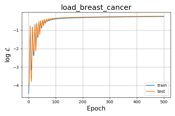
Fig. 6 Log-likelihood of logistic model over training epoch for the load_breast_cancer dataset.

which is great as both the train and test datasets have similar \(\mathcal{L}\) values over epochs even though we are only using the training data. We can safely say we are not overfitting nor underfitting for this particular setting.

A quick animation of our model predictions for the test data shows that we achieve a final accuracy of \(\approx90\)!

Playback problem? Try here
Vid. 1 Logistic regression predictions over training epochs.

Multiclass Classification

So far we have only talked about two classes. If we have more than two classes and each observation can strictly belong to a single class, we will need to change our \(\phi\) function to the softmax function. The update rules for our weights and bias parameters remain the same as stated in Eq. \(\eqref{eq:w}\) and Eq. \(\eqref{eq:b}\) as shown in Eq. (33) from classification#multiclass.

Softmax and categorical cross entropy loss functions

def softmax(z):
    """ Softmax function """
    e = np.exp(z - z.max(axis = -1, keepdims = True))
    return e / e.sum(axis = -1, keepdims = True)

def categorical_cross_entropy(y_true, y_pred):
    """ Categorical cross entropy objective function """
    offset = 1e-8 # To ensure we never compute log(0) as this is not defined!
    return np.log(y_pred[np.where(y_true == 1)] + offset).sum() / len(y_true)

Example 2: Multiclass classification with load_iris

The load_iris dataset is an easy multiclass classification dataset whereby the task is to classify each observation into one of three classes.

Dataset

load_iris

Data Set Characteristics:

Number of Instances: 150 (50 in each of three classes)

Number of Attributes: 4 numeric, predictive attributes and the class

Attribute Information:

• sepal length in cm

• sepal width in cm

• petal length in cm

• petal width in cm

• class:

  • Iris-Setosa

  • Iris-Versicolour

  • Iris-Virginica

Summary Statistics

sepal length:	4.3	7.9	5.84	0.83	0.7826
sepal width:	2.0	4.4	3.05	0.43	-0.4194
petal length:	1.0	6.9	3.76	1.76	0.9490 (high!)
petal width:	0.1	2.5	1.20	0.76	0.9565 (high!)

Missing Attribute Values: None Class Distribution: 33.3% for each of 3 classes. Creator: R.A. Fisher Donor: Michael Marshall (MARSHALL%PLU@io.arc.nasa.gov) Date: July, 1988

The famous Iris database, first used by Sir R.A. Fisher. The dataset is taken from Fisher’s paper. Note that it’s the same as in R, but not as in the UCI Machine Learning Repository, which has two wrong data points.

This is perhaps the best known database to be found in the pattern recognition literature. Fisher’s paper is a classic in the field and is referenced frequently to this day. (See Duda & Hart, for example.) The data set contains 3 classes of 50 instances each, where each class refers to a type of iris plant. One class is linearly separable from the other 2; the latter are NOT linearly separable from each other.

References

• Fisher, R.A. “The use of multiple measurements in taxonomic problems” Annual Eugenics, 7, Part II, 179-188 (1936); also in “Contributions to Mathematical Statistics” (John Wiley, NY, 1950).

• Duda, R.O., & Hart, P.E. (1973) Pattern Classification and Scene Analysis. (Q327.D83) John Wiley & Sons. ISBN 0-471-22361-1. See page 218.

• Dasarathy, B.V. (1980) “Nosing Around the Neighborhood: A New System Structure and Classification Rule for Recognition in Partially Exposed Environments”. IEEE Transactions on Pattern Analysis and Machine Intelligence, Vol. PAMI-2, No. 1, 67-71.

• Gates, G.W. (1972) “The Reduced Nearest Neighbor Rule”. IEEE Transactions on Information Theory, May 1972, 431-433.

• See also: 1988 MLC Proceedings, 54-64. Cheeseman et al”s AUTOCLASS II conceptual clustering system finds 3 classes in the data.

• Many, many more …

Independent Sigmoid Classifiers

Fitting a binary Logistic Regression model to each class in the load_iris dataset

data = ds.load_iris()
X, y = data['data'], data['target']
y    = np.eye(len(np.unique(y)))[y] # one-hot encode

# # Print description
# print(data['DESCR'])

X_train, X_test, y_train, y_test = train_test_split(X, y, test_size = 0.2, random_state = 2020)

L = []
Z = []

for j in range(3):
    model = LogisticRegression(binary_cross_entropy, sigmoid, random_state = 2020).fit(X_train, y_train[:,j], X_test, y_test[:,j], alpha = 1e-3, epochs = 1000)

    L.append(model.logs['L'])
    Z.append(model.logs['Zs'])

L, Z = map(lambda A : np.moveaxis(A, 0, -1), [L, Z])

L    = L.sum(axis = -1)

Conveniently our test set has an equal distribution of the three classes (10 observations each). Plotting the variable L yields

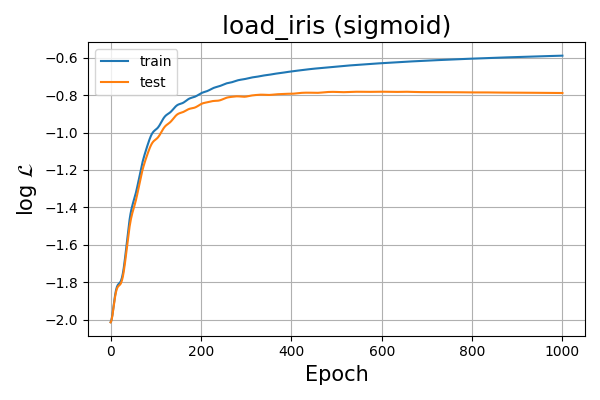
Fig. 7 Log-likelihood of sigmoid logistic model over training epoch for the load_iris dataset.

which looks like we have converged if we observe the test set. Taking a closer look at our model predictions over time we have

Playback problem? Try here
Vid. 2 Sigmoid logistic regression latent space over training epochs.

The above visualisation maps our 3D \(\mathbf{\hat{Y}}\) to a 2D space by having at each corner of the triangle, the probability of belonging to that class being 1, whilst the probability of belonging to any other class strictly \(0\). Anywhere inbetween will map to somewhere within the triangle. Each circle represent a datapoint and the colour of that circle represents the true \(\mathbf{Y}\). If our estimate is 100% correct, then each circle will belong to the same coloured region.

As the animation ends, we see that there is no correlation between the red and green classes but both have the potential to be misclassified as the blue class. Two of the blue classes were misclassified as being green.

Softmax Classifier

Fitting a softmax Logistic Regression model to the load_iris dataset

data = ds.load_iris()
X, y = data['data'], data['target']
y    = np.eye(len(np.unique(y)))[y] # one-hot encode

# # Print description
# print(data['DESCR'])

X_train, X_test, y_train, y_test = train_test_split(X, y, test_size = 0.2, random_state = 2020)

model = LogisticRegression(categorical_cross_entropy, softmax, random_state = 2020).fit(X_train, y_train, X_test, y_test, alpha = 1e-3, epochs = 1000)

L = model.logs['L']
Z = model.logs['Zs']

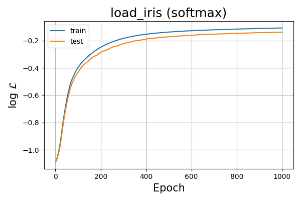
Fig. 8 Log-likelihood of softmax logistic model over training epoch for the load_iris dataset.

Playback problem? Try here
Vid. 3 Softmax logistic regression latent space over training epochs.

We observe that the \(\log \mathcal{L}\) values are much better for the softmax classifier than the binary sigmoid classifier. Observing the latent space projection videos, we see that generally the softmax classifier has points closer to the corners of the triangle implying it is more sure of it’s predictions albeit the same mis-classification.