k-Nearest Neighbours
The \(k\)-Nearest Neighbours (k-NN) is a simple yet effective algorithm for regression and classificaion tasks (with identical code for each task). The k-NN algorithm is a non-parametric method proposed by Thomas Cover 1. Essentially, we use a similarity measure between some query point \(\mathbf{x}^{*}\) and some training data \(\mathbf{X}\) to predict the associated target value(s). As usual, assume that our dataset \(\mathbf{X}\in\mathbb{R}^{n,m}\) and \(\mathbf{Y}\in\mathbb{R}^{n,c}\) where \(n\) is the number of observations, \(m\) is the number of features, and \(c\) is the number of targets.
Note
The similarity measure we use is known as the Minkowski distance and is defined by:
Essentially, Eq. \(\eqref{eq:minkowski}\) is defined by the vector \(p\)-norm so the Minkowski distance and \(p\)-norm are synonymous.
Regression
For visual aid, lets consider a one-dimensional toy problem. Lets generate the observations \(x\sim U(0,2\pi)\) and the targets \(y|x\sim\mathcal{N}(\sin(x),\epsilon^2)\) where we set \(\epsilon=0.3\) and group them into a train, validation, and test datasets.
Python
Generating synthetic regression data
# Vital imports
from   sklearn.model_selection import train_test_split
import numpy as np

# Reproducibility
np.random.seed(2020)

N = 200 # Total number of points
n = 50  # Total number of samples
X = np.linspace(0, 2 * np.pi, N).reshape(-1, 1)
T = np.sin(X)

# Sample random indices to be our data
r = np.random.choice(N, size = n)
x = X[r]
t = T[r]
y = t + np.random.normal(scale = 0.3, size = t.shape) # Add noise to observations

# Train / Val / Test
x_train, x_test, y_train, y_test = train_test_split(x, y)
x_train, x_val , y_train, y_val  = train_test_split(x_train, y_train)

train = x_train, y_train
val   = x_val  , y_val
test  = x_test , y_test
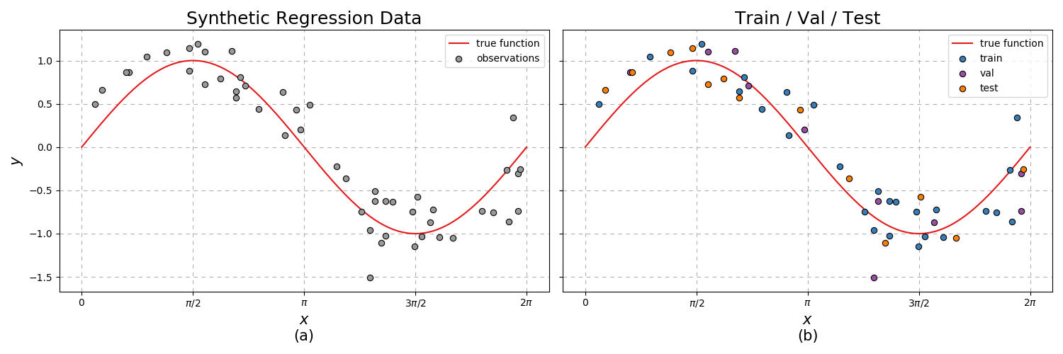
Fig. 9 (a) Generated noisy \(\sin\) function. (b) Train / validation / test split.
As the algorithm name suggests, when querying a new data point in observation space, we use the \(k\) nearest data points in observation space to predict in target space.
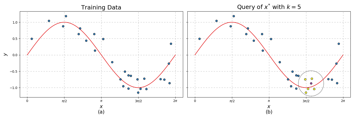
Fig. 10 (a) Training data. (b) Example new query point (purple) using the 5 nearest neighbours from the train for inference.
Python
Coding of Eq. \({\eqref{eq:minkowski}}\)
def numpy_distance_neighbours(X1, X2, k, p):
    """ Computes the k-nearest distances and neighbours based on the numpy implementation of the minkowski distance """
    distances  = np.power(np.sum(np.power(np.fabs(X1[:,None] - X2[None,:]), p), axis = -1), 1 / p)
    neighbours = distances.argsort(axis = 1)[:,:k]
    rows       = np.arange(len(distances))[:,None]
    return distances[rows, neighbours], neighbours
Python
k-Nearest Neighbours Class
class kNearestNeighbours():
    """
    k-Nearest Neighbours class

    Parameters
    =============
        k        : int
                   Number of neighbours to consider when running model inference.

        p        : int, float [1, \infty]
                   The p parameter in the Minkowski distance metric.

        weighted : bool
                   If True, weight neighbours by their inverse distance.

        func     : function
                   Function call to use to compute the k-nearest distances and neighbours.
    """
    def __init__(self, k = 5, p = 2, weighted = True, func = numpy_distance_neighbours):
        self._params = dict(k = k, p = p, weighted = weighted)
        self.__func  = func

    def fit(self, X, y):
        self.X = X
        self.y = y
        return self

    def __call__(self, X):
        distances, neighbours = self.__func(X, self.X, k = self._params['k'], p = self._params['p'])
        if self._params['weighted']:
            is0             = np.where(distances == 0)                    # find where the distance is 0
            distances[is0]  = 1
            weights         = 1 / distances                               # weight by inverse distance
            weights[is0[0]] = 0                                           # zero out all rows that had initially 0 distance
            weights[is0]    = 1                                           # correct inverse weights to be 1 where distance is 0
            weights        /= weights.sum(axis = 1, keepdims = True)      # ensure that weights sum to 1
        else:
            weights         = np.ones_like(distances) / self._params['k']
        weights.resize(*weights.shape, 1)
        return (weights * self.y[neighbours]).sum(axis = 1)

    def rmse(self, *data):
        return [np.sqrt(np.mean((np.square(self(X) - y)))) for (X, y) in data]
Python
Model results on toy regression data
k_range       = range(1, 13)
rmse_uniform  = [kNearestNeighbours(k = k, weighted = False).fit(x_train, y_train).rmse(train, val, test) for k in k_range]
rmse_weighted = [kNearestNeighbours(k = k, weighted = True ).fit(x_train, y_train).rmse(train, val, test) for k in k_range]
Plotting the rmse results yields the following plot.
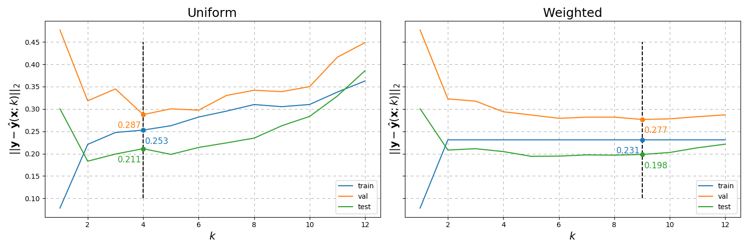
Fig. 11 RMSE results of toy regression data over the number of neighbours \(k\) with constant \(p=2\).
Not bad! The scatter points along the black dashed line represent the results when the validation error is minimised. It is normal practice to choose the model that minimises the validation data whilst training on the training data. We see that the weighted solution has marginally better results. Lets try the same code on a more realistic regression problem - the load_boston dataset.
Dataset
load_boston
Data Set Characteristics:
- Number of Instances
506
- Number of Attributes
13 numeric/categorical predictive. Median Value (attribute 14) is usually the target.
- Attribute Information (in order)
CRIM per capita crime rate by town
ZN proportion of residential land zoned for lots over 25,000 sq.ft.
INDUS proportion of non-retail business acres per town
CHAS Charles River dummy variable (= 1 if tract bounds river; 0 otherwise)
NOX nitric oxides concentration (parts per 10 million)
RM average number of rooms per dwelling
AGE proportion of owner-occupied units built prior to 1940
DIS weighted distances to five Boston employment centres
RAD index of accessibility to radial highways
TAX full-value property-tax rate per $10,000
PTRATIO pupil-teacher ratio by town
B 1000(Bk - 0.63)^2 where Bk is the proportion of blacks by town
LSTAT % lower status of the population
MEDV Median value of owner-occupied homes in $1000’s
- Missing Attribute Values
None
- Creator
Harrison, D. and Rubinfeld, D.L.
This is a copy of UCI ML housing dataset. https://archive.ics.uci.edu/ml/machine-learning-databases/housing/
This dataset was taken from the StatLib library which is maintained at Carnegie Mellon University.
The Boston house-price data of Harrison, D. and Rubinfeld, D.L. ‘Hedonic prices and the demand for clean air’, J. Environ. Economics & Management, vol.5, 81-102, 1978. Used in Belsley, Kuh & Welsch, ‘Regression diagnostics …’, Wiley, 1980. N.B. Various transformations are used in the table on pages 244-261 of the latter.
The Boston house-price data has been used in many machine learning papers that address regression problems.
Belsley, Kuh & Welsch, ‘Regression diagnostics: Identifying Influential Data and Sources of Collinearity’, Wiley, 1980. 244-261.
Quinlan,R. (1993). Combining Instance-Based and Model-Based Learning. In Proceedings on the Tenth International Conference of Machine Learning, 236-243, University of Massachusetts, Amherst. Morgan Kaufmann.
Python
Loading sklearn’s load_boston dataset
from sklearn.datasets      import load_boston
from sklearn.preprocessing import StandardScalar()

X, y = load_boston(return_X_y = True)
y    = y.reshape(-1, 1)

def train_val_test_split(X, y, *args, **kwargs):
    X_train, X_test, y_train, y_test = train_test_split(X      , y      , *args, **kwargs)
    X_train, X_val , y_train, y_val  = train_test_split(X_train, y_train, *args, **kwargs)
    return X_train, X_val, X_test, y_train, y_val, y_test, (X_train, y_train), (X_val, y_val), (X_test, y_test)

X_train, X_val, X_test, y_train, y_val, y_test, train, val, test = train_val_test_split(X, y, random_state = 2020)

# scale values so each dimension has an equal say when computing the Minkowski distances
scaler = StandardScaler().fit(X_train)

X_train, X_test = scaler.transform(X_train), scaler.transform(X_test)

del X, y
Python
Model results on the load_boston data
k_range       = range(1, len(X_train))
rmse_uniform  = [kNearestNeighbours(k = k, weighted = False).fit(X_train, y_train).rmse(train, val, test) for k in k_range]
rmse_weighted = [kNearestNeighbours(k = k, weighted = True ).fit(X_train, y_train).rmse(train, val, test) for k in k_range]
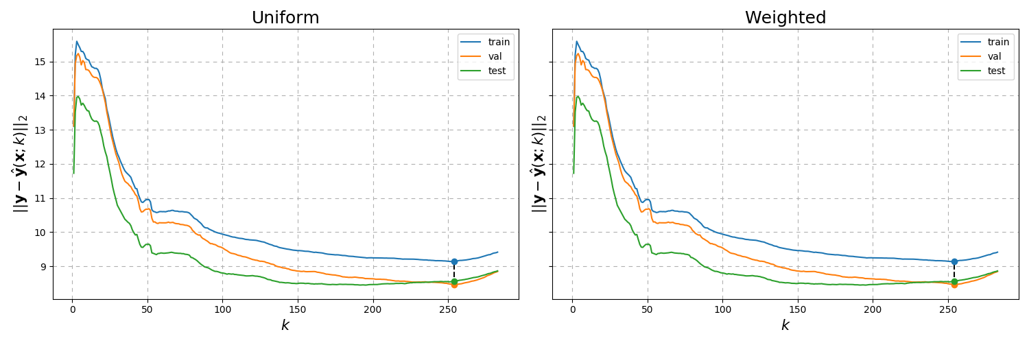
Fig. 12 RMSE results of the load_boston data over the number of neighbours \(k\) with constant \(p=2\).
From the above plots, it seems that both the uniform and weighted cases yield the same errors. Lets try varying \(p\) to see if they really are the same.
Python
Model results on the load_boston data varying \(p\)
rmse_1 = [kNearestNeighbours(k = k, weighted = True, p = 1).fit(X_train, y_train).rmse(train, val, test) for k in k_range]
rmse_2 = [kNearestNeighbours(k = k, weighted = True, p = 2).fit(X_train, y_train).rmse(train, val, test) for k in k_range]
rmse_3 = [kNearestNeighbours(k = k, weighted = True, p = 3).fit(X_train, y_train).rmse(train, val, test) for k in k_range]
rmse_4 = [kNearestNeighbours(k = k, weighted = True, p = 4).fit(X_train, y_train).rmse(train, val, test) for k in k_range]
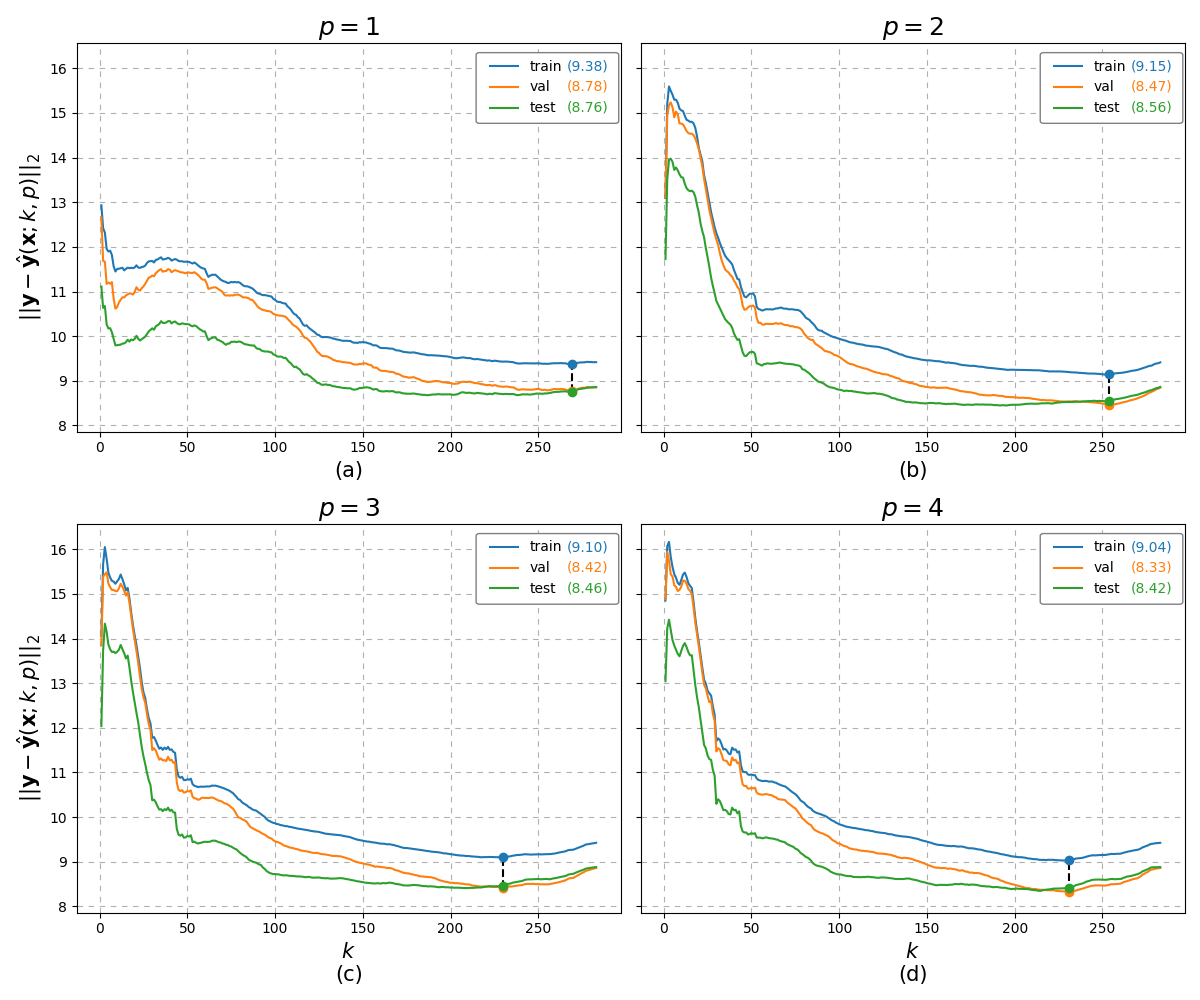
Fig. 13 RMSE results of the load_boston data over the number of neighbours :k and Minkowski distance parameter \(p\).
From the above, we can see that as \(p\) varies, the curves do change with slightly different optimal results with the trend that the RMSE values decrease as \(p\) increases. Running this code however proves to be slow so lets look at how we can make the code more efficient for our use case. One route may be to simply do the same code in another language i.e. C and see how that provides a speed up. Alternatively, we can consider partitioning the \(m\) dimensional observation data space into a k-dimensional trees <https://en.wikipedia.org/wiki/K-d_tree>. Lets see how the numpy, C, and KDTree implementations costs in terms of time to run.
Python
Implementations of Nearest Neighbours
from time                     import time as _time

from sklearn.spatial.distance import cdist
from sklearn.spatial          import cKDTree

def timeit(func, *args, n_iterations = 1000):
    """ Times the function func, with parsed args and returns the n_iterations worth of times in seconds """
    times = np.empty(n_iterations)
    for i in range(n_iterations):
        start    = _time()
        func(*args)
        times[i] = _time() - start
    return times

def numpy_distance_neighbours(X1, X2, k, p):
    """ Computes the k-nearest distances and neighbours based on the numpy implementation of the minkowski distance """
    distances  = np.power(np.sum(np.power(np.fabs(X1[:,None] - X2[None,:]), p), axis = -1), 1 / p)
    neighbours = distances.argsort(axis = 1)[:,:k]
    rows       = np.arange(len(distances))[:,None]
    return distances[rows, neighbours], neighbours

def cdist_distance_neighbours(X1, X2, k, p):
    """ Computes the k-nearest distances and neighbours based on the c implementation of the minkowski distance """
    distances  = cdist(X1, X2, metric = 'minkowski', p = p)
    neighbours = distances.argsort(axis = 1)[:,:k]
    rows       = np.arange(len(distances))[:,None]
    return distances[rows, neighbours], neighbours

def ckdtree_distance_neighbours(X1, X2, k, p):
    """ Computes the k-nearest distances and neighbours using the c implementation of the KD Tree """
    distances, neighbours = cKDTree(X2).query(X1, k = k, p = p, n_jobs = -1)
    if k == 1:
        distances, neighbours = distances.reshape(-1, 1), neighbours.reshape(-1, 1)
    return distances, neighbours


numpy_time  = timeit(numpy_distance_neighbours  , X_train, X_test, 2, 2)
cdist_time  = timeit(cdist_distance_neighbours  , X_train, X_test, 2, 2)
kdtree_time = timeit(ckdtree_distance_neighbours, X_train, X_test, 2, 2)
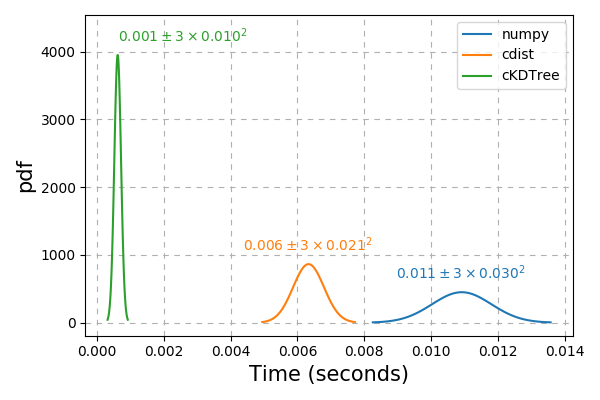
Fig. 14 Time cost of computing the nearest neighbours and distances across different implementations.
From the above, it is clear that the k-d tree method is the fastest of the three with the C implementation already being a significant improvement over the numpy implementation. We redefine our earlier defined class implementation with the k-d tree method.
Python
Efficient implementation of k-Nearest Neighbours Class
class kNearestNeighbours():
    """
    k-Nearest Neighbours class

    Parameters
    =============
        k        : int
                   Number of neighbours to consider when running model inference.

        p        : int, float [1, \infty]
                   The p parameter in the Minkowski distance metric.

        weighted : bool
                   If True, weight neighbours by their inverse distance.
    """
    def __init__(self, k = 5, p = 2, weighted = True):
        self._params = dict(k = k, p = p, weighted = weighted)

    def fit(self, X, y):
        self.cKDTree = cKDTree(X).query
        self.y       = y
        return self

    def __call__(self, X):
        distances, neighbours = self.cKDTree(X, k = self._params['k'], p = self._params['p'], n_jobs = -1)
        if self._params['k'] == 1:
            distances, neighbours = distances.reshape(-1, 1), neighbours.reshape(-1, 1)
        if self._params['weighted']:
            is0             = np.where(distances == 0)
            distances[is0]  = 1
            weights         = 1 / distances
            weights[is0[0]] = 0
            weights[is0]    = 1
            weights        /= weights.sum(axis = 1, keepdims = True)
        else:
            weights         = np.ones_like(distances) / self._params['k']
        weights.resize(*weights.shape, 1)
        return (weights * self.y[neighbours]).sum(axis = 1)

    def rmse(self, *data):
        return [np.sqrt(np.mean((np.square(self(X) - y)))) for (X, y) in data]

    def acc(self, *data):
        return [(self(X).round(0) == y).mean() for (X, y) in data]
Classification
In this section we consider the target variable \(\mathbf{y}\in\{0,1\}^n\) i.e. the binary classification problem. This is easily extendible to the case where there are more than two classes. We now generate a toy non-linear boundaried classification problem below. The toy problem has the target variable dependent on a two dimensional observation. \(x_1\overset{\text{iid}}{\sim} U(0,1)\), \(x_2\overset{\text{iid}}{\sim} U(0,1)\) and \(p(y=1|x_1,x_2) = p\big(\sqrt{x_1^2 + x_2^2} - r > \epsilon\big)\) where we set \(r = 0.8\) and \(\epsilon\overset{\text{iid}}{\sim}\mathcal{N}(0, 0.2^2)\).
Python
Generating synthetic classification data
# radius of boundary
r = 0.8

def gen_classification(n, random_state = None):
    np.random.seed(random_state)

    x1 = np.random.uniform(size = n)
    x2 = np.random.uniform(size = n)
    X  = np.c_[x1, x2]
    y = np.sqrt(x1 ** 2 + x2 ** 2 + np.random.normal(scale = 0.2, size = n)) > r
    y = y.astype(int).reshape(n, 1)
    return X, y

x = np.linspace(0, r, 100)
b = np.sqrt(r ** 2 - x ** 2) # boundary

X, y = gen_classification(500, random_state = 2020)
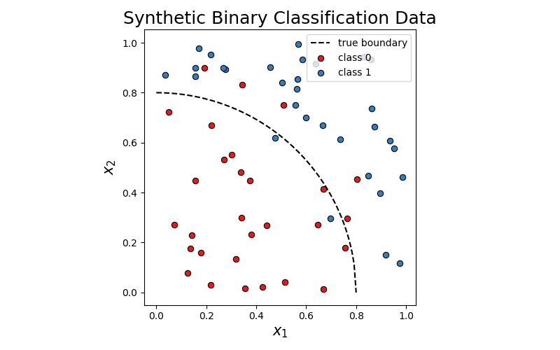
Fig. 15 Generated classification data. The classes have been noisily assigned if the distance from the origin is more than 0.8 or not. For less cluttered visual display, only the first 60 scatter points have been visualised.
Python
Model results on toy classification data
train = X_train, y_train
val   = X_val  , y_val
test  = X_test , y_test

rmse_uniform  = []
acc_uniform   = []

rmse_weighted = []
acc_weighted  = []

for k in range(1, len(X_train)):
    model = kNearestNeighbours(k = k).fit(X_train, y_train)
    rmse_uniform.append(model.rmse(train, val, test))
    acc_uniform.append(model.acc(train, val, test))

    model = kNearestNeighbours(k = k, weighted = True).fit(X_train, y_train)
    rmse_weighted.append(model.rmse(train, val, test))
    acc_weighted.append(model.acc(train, val, test))
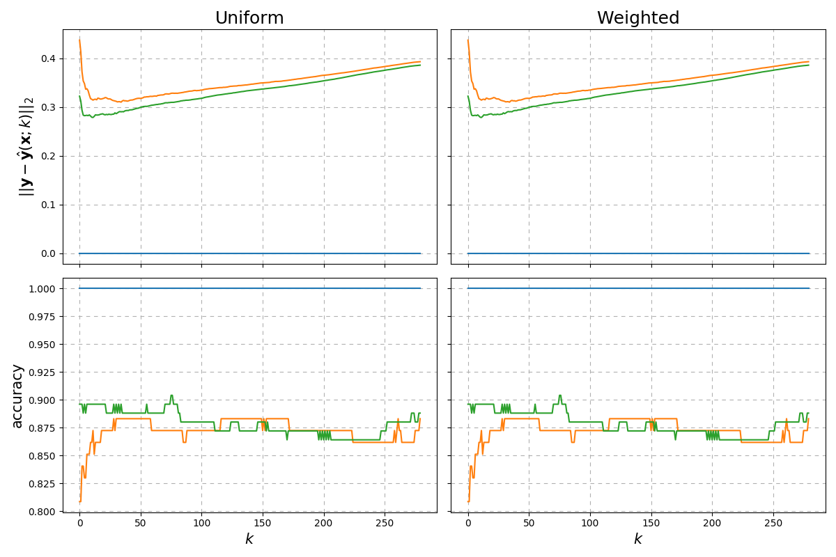
Fig. 16 RMSE and accuracy results of fitting a \(k\)-NN to the toy classication data over the number of neighbours \(k\) with constant \(p=2\).
A similar analysis can be done where we vary \(p\) yielding the below.
Python
Model results on the toy classification data varying \(p\)
p_range = range(1, 5)
k_range = range(1, len(X_train))

results = dict(rmse = {}, acc = {})
for p in p_range:
    rmse = results['rmse'][p] = []
    acc  = results['acc' ][p] = []
    for k in k_range:
        model = kNearestNeighbours(k = k, weighted = True, p = p).fit(X_train, y_train)
        rmse.append(model.rmse(train, val, test))
        acc.append(model.acc(train, val, test))
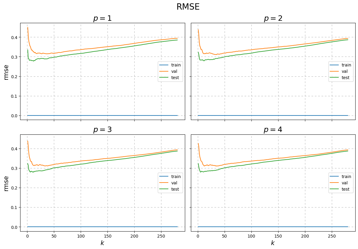
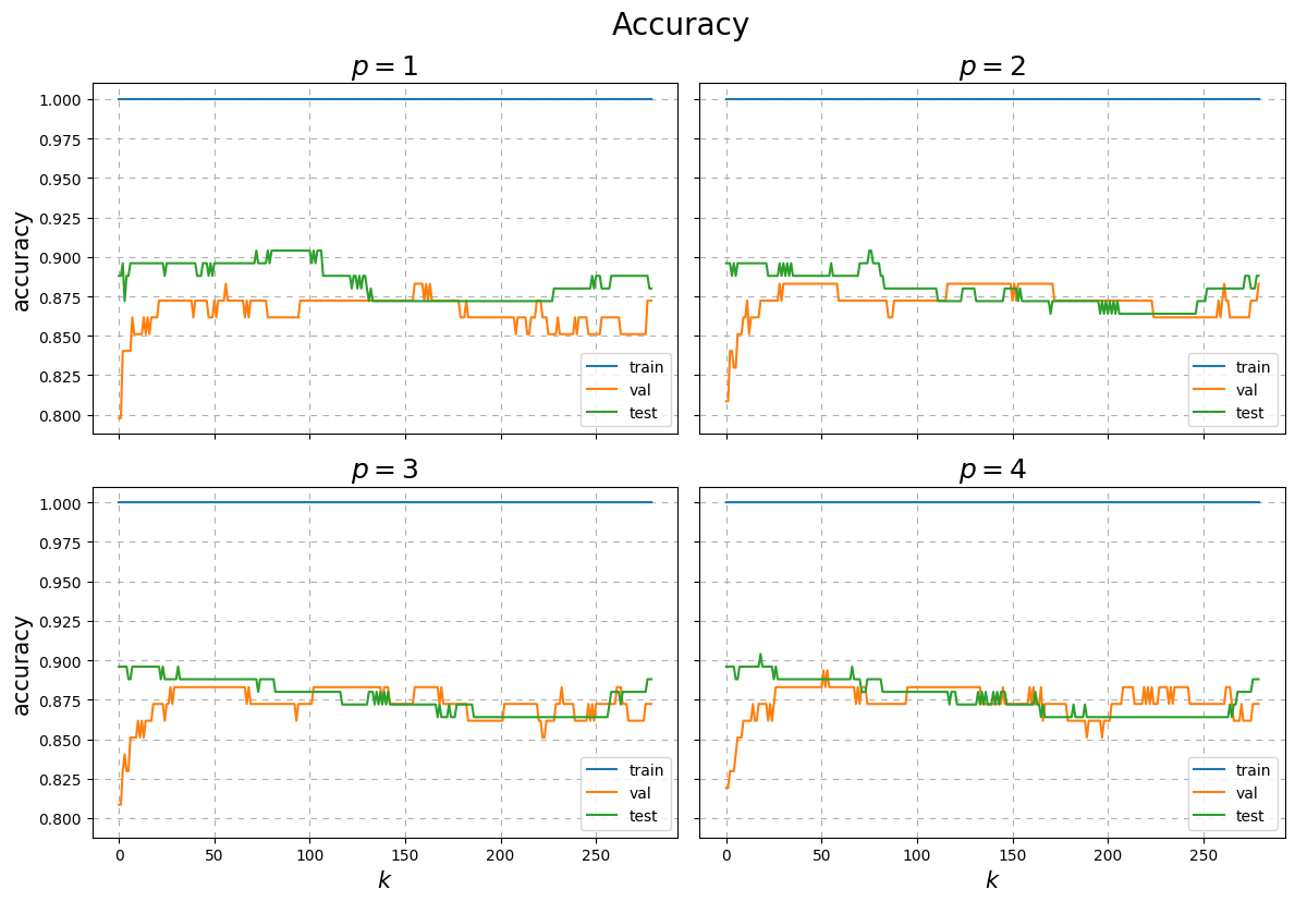
Fig. 17 RMSE and accuracy results of fitting a \(k\)-NN to the toy classication data over the number of neighbours \(k\) with varying \(p\).
- 1
Cover, P. Hart, Nearest Neighbor Pattern Classification, 1967, https://ieeexplore.ieee.org/document/1053964?arnumber=1053964