Introduction
New to Reinforcement Learning (RL)? This series of tutorials aims to get you up to speed with the foundations of RL. It is assumed you know the machine learning techniques involved here i.e. gradient based optimisation for both linear and non-linear modelling. If you are unsure of these concepts, please visit my How to: Machine Learning <../how-to-ml/index.html> tutorial series. Enough with the prerequisites, lets have a look at what problems falls under RL and how to generally find the solutions.
Problem Setup
There are two distinct components in reinforcement learning. The first is an environment we are trying to understand. In Mathematics the environment is a (stochastic) system which requires a decision making process. The other component is the agent which is the brains behind the decision making process. The reinforcement learning framework is really about formulating, and then training the agent. Popular examples of environments are board games and arcade games. This has been somewhat extended to recommender systems, robotics and automous systems but it is still far too incomplete for a lot of practial problems i.e. self-driving cars.
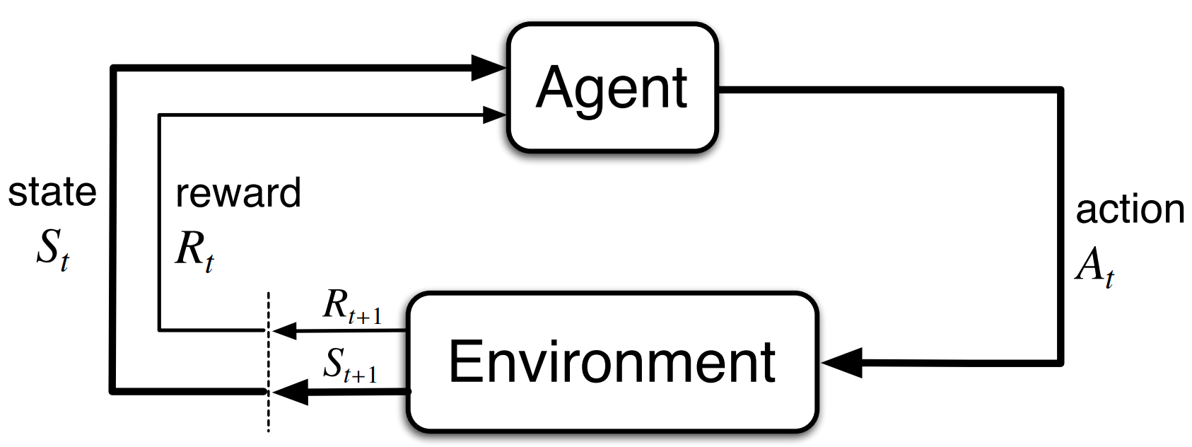
Fig. 35 The agent-environment interaction in a MDP. Image courtesy of Reinforcement Learning: An Introduction, p38, R. Sutton & A. Barto (2017).
The process involves the environment and agent taking turns where the agent observes some state that is given by the environment to then choose some action, and the environment generates a reward signal and next state given the agent’s action and the current state. Now lets go through some notation on how the process starts. Suppose we initialise both the environment and agent. Denoting the state space \(\mathcal{S}\) and the action space \(\mathcal{A}\), the agent observes we are in some state \(S_0\sim\mathcal{S}_\text{initial}\subseteq\mathcal{S}\). The agent then draws an action according to \(A_0\sim\pi(S_0)\) where \(\pi : \mathcal{S} \rightarrow \mathcal{A}\) (i.e. \(\pi(S_0)\) is the probability distribution over \(\mathcal{A}\) conditioned on the current state \(S_0\)), and the environment outputs the reward signal \(R_1\) and next state \(S_1\). Note that all letters used here are capital and thereby is referring to states, actions, and rewards as random variables. The agent needs to use these reward signals to learn which actions were good or bad.
Value Function
Measuring how good a state is can be thought of as the expected total return you think you can get from the given state. Mathematically, let us define the expected total return if we followed the policy \(\pi\) to be \(\text{R}^\pi(S) := \mathbb{E}_\pi[\sum_{j=t}^\infty R_j\mid S_t = S]\). If we take a step back and think of tasks that terminate only when some objective is failed i.e. balance a pen by putting the tip on your hand, we may not have a finite \(\text{R}^\pi(S)\) e.g. \(R_t = 1\ \ \forall\ \ t\) s.t. the pen is still balancing, otherwise \(R_t = 0\). It is from this stance we justify a discount parameter, \(\gamma\in[0,1]\), to control how short or far sighted we want to be. Quantifying the expected total discounted return is the well known Value function in the field,
where \(S'\) is the state after being in state \(S\) and taking an action \(A\) according to the policy \(\pi(S)\). Though we can define the Value function as per Eq. \(\eqref{eq:V1}\), we can write it as Eq. \(\eqref{eq:V2}\) by writing the expected sum to be the first term and all proceeding terms. This means to quantify how good a state is becomes easier as we can rely on dynamic programming techniques i.e. instead of computing a (possibly) infinite sum for every state as stated in Eq. \(\eqref{eq:V1}\), we can instead say the Value of a state is simply the addition of the expected immediate reward and the discount factor multiplied by the expected Value of the next state. Though we may have defined how good a state can be, we need to think about how we can visit these states to reap the rewards! This calls for a Action-Value function!
Action-Value Function
The Action-Value Function, often referred to as the \(Q\) value function in the RL, measures how good being in a particular state and taking a particular action is. Lets go through an example of this below.
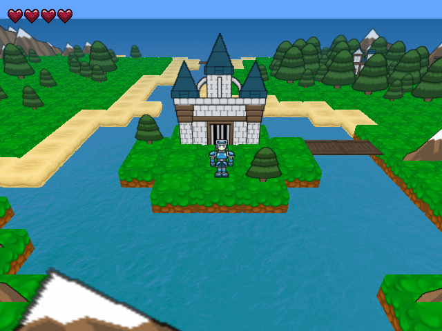
Fig. 36 Example 2D top down terrain game. Image courtesy of The Hero’s Journey.
If we imagine ourselves as the character in the image above, and the objective is to enter the castle, we notice going up is the obvious move. If we attempt to go right, we remain in the same location and have wasted a single timestep. If we attempt to go down, we may lose a heart (assuming we cannot swim with all that heavy armour!). If we go left, then we go further away from the objective as we need to come back to the current state before going up. In this example the state is the current location of the character, the actions are up, right, down, and left and \(Q^\pi(S,\cdot)\) values could be \((9, 8, -11, 7)\) if we assume \(+10\) for reaching the goal, \(-10\) for entering the water, and a \(-1\) cost per action.
The relationship between \(V^\pi(S)\) and \(Q^\pi(S,A)\) is
which makes sense as if we follow the optimal path defined by our policy which in turn is defined by taking the action with the highest \(Q\) value at every state, we should yield a good expected total discounted return which is the Value function. Coming back to our example vector of \(Q^\pi(S,\cdot) = (9, 8, -11, 7)\), we have in this example \(V^\pi(S) = 9\).
Now that we are equipped with the foundations of how to measure the goodness of a state and how to navigate through the state space by considering the state-action pair, we are set to look at methods for learning \(V^\pi,\ Q^\pi\), or even \(\pi\) directly.