Random Forest

The Random Forest is an ensemble method for both regression and classification tasks. It works by taking an average of a collection of weaker Decision trees. So first we need to understand a single Decision tree, how to make it weaker and then aggregate a collection of these to a Random Forest.

Decision Tree

The Decision tree algorithm is a partitioning algorithm that queries an observation \(\mathbf{x}_i\in\mathbb{R}^m\) and based on these queries will provide some estimator of the associated target value. The Decision tree can be visualised as a collection of query nodes each containing two branches and eventually ending up at a leaf node which has no branches.

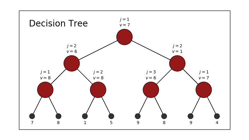
Fig. 18 Example diagram of a Decision Tree. We start from the top red query node where \(j\) indicates the feature to be queried and \(v\) the value to be queried. If True, traverse left otherwise, traverse right until you reach a grey leaf node which represents \(\hat{y}\).

Example use of a Decision Tree

Consider \(\mathbf{x} = [8, 0, 5]\). Using the above Fig. 18 we would

• query \(8 \leq 7 \Rightarrow\) False so we traverse right

• query \(0 \leq 1 \Rightarrow\) True so we traverse left

• query \(5 \leq 6 \Rightarrow\) True so we end up with \(\hat{y} = 9\)

The challenge is to come up with the queries that bests partition the data such that we can provide the best estimator for the target values. Normally we act greedily based on some objective function to decide which of the \(m\) features should be queried and what value \(v\) should be considered for the query. For simplicity we will consider two objectives - one for regression, and one for classification. Similarly, we can define a leaf function which is used at a leaf node within our Decision Tree. The two most popular objective function for each task is variance and entropy respectively. Mathematically, they are both defined as

\begin{align} V(y) &= \frac{1}{n}\sum_{i=1}^n (y_i - \bar{y})^2\\\nonumber\\ \mathcal{E}(p) &= \sum_{i=1}^n -p_i \log p_i \end{align}

As we will later weight these functions by the number of samples are present, we can multiply both equations by \(n\). Below we implement the objective and leaf functions.

Python

Decision Tree Objectives

def variance(y):
    """ Computes the weighted variance """
    return np.square(y - y.mean()).sum()

def entropy(y):
    """ Computes the weighted entropy """
    n = len(y)
    p = np.unique(y, return_counts = True)[1] / n
    return -p @ np.log(p) * n

Leaf Functions

def average(y):
    """ Computes the average """
    return np.mean(y, axis = 0)

def proportion(c):
    """ Returns proportion leaf function """

    def _proportion(y):
        """ Computes the proportion of class appearance """
        return np.eye(c)[y].mean(axis = 0)

    # enables function to be computed in parallel if named the same
    _proportion.__qualname__ = f'proportion{c}'

    return _proportion

As we will try both a regression and classifcation task lets define a Metrics class to help us.

Python

Metrics Class

class Metrics():
    """
    Metrics class

    To be inherited by algorithms for regression and classification tasks.
    """
    def rmse(self, *data, **kwargs):
        """ Root Mean-Squared Error (Regression)"""
        return np.array([np.sqrt(np.mean(np.square(self(X, **kwargs) - y))) for (X, y) in data])

    def acc(self, *data, **kwargs):
        """ Accuracy (Classification) """
        ret = []
        for (X, Y) in data:
            hat = self(X, **kwargs).argmax(axis = 1)
            y   = Y.argmax(axis = 1) if Y.ndim == 2 else Y
            ret.append((hat == y).mean())
        return np.array(ret)

    def confusion_matrix(self, *data, **kwargs):
        """ Confusion Matrix (Clasification) """
        ret = []
        for (X, Y) in data:
            hat  = self(X, **kwargs).argmax(axis = 1)
            y    = Y.argmax(axis = 1) if Y.ndim == 2 else Y
            u    = np.unique(y)
            c    = len(u)
            conf = np.empty((c, c))
            for i in range(c):
                for j in range(c):
                    conf[i,j] = ((y == u[i]) & (hat == u[j])).mean()
            ret.append(conf)
        return np.array(ret)

Finally, using the code so far, we can look at implementing the Decision Tree class.

Python

Decision Tree Class

class DecisionTree(Metrics):
    """
    Decision Tree class

    Parameters
    ==============
        objective : function
                    Objective function to minimise when fitting.

        leaf      : function
                    Leaf function to use when at a leaf node.

        max_depth : int
                    Maximum depth level.
    """
    def __init__(self, objective, leaf, max_depth = np.inf):
        self._params   = dict(objective = objective, leaf = leaf, max_depth = max_depth)

    def fit(self, X, y, depth = 0):

        # precompute the leaf value
        leaf = self._params['leaf'](y)

        # stopping condition
        #   • max depth has been reached
        #   • there is only a single unique value
        if depth == self._params['max_depth'] or len(np.unique(y)) == 1:
            return dict(leaf = leaf)

        # exhaustive search
        best = np.inf
        for j, x in enumerate(X.T):
            ux = np.unique(x)
            for v in ux[:-1]:
                mask  = x <= v
                score = self._params['objective'](y[mask]) + self._params['objective'](y[~mask])
                if score < best:
                    best = score
                    tree = dict(mask = mask, v = v, j = j, leaf = leaf)

        # stopping condition
        #  • only a single unique x vector
        if best == np.inf:
            return dict(leaf = leaf)

        # get rid of "mask" from the tree to save memory
        mask      = tree.pop('mask')

        # recursively call on the "left" and "right" branches
        tree['l'] = self.fit(X[ mask], y[ mask], depth + 1)
        tree['r'] = self.fit(X[~mask], y[~mask], depth + 1)

        # if at the root node, save the entire tree, otherwise return this branch onwards
        if depth:
            return tree
        self.tree = tree
        return self

    def _predict_one(self, x, prune = np.inf):
        """ Helper function that predicts a single x vector """
        tree  = self.tree
        depth = 0
        while 'l' in tree:
            tree   = tree['l'] if x[tree['j']] <= tree['v'] else tree['r']
            depth += 1

            # prune tree to evaluate as though max_depth = prune when trained
            if depth == prune: break
        return tree['leaf']

    def __call__(self, X, **kwargs):
        return np.array([self._predict_one(x, **kwargs) for x in X])

Note

We can think of the max_depth parameter as a regularisation parameter. The lower it is, the more likely it does not overfit to the noise in the training data.

Caution

This is not an exhaustive list of parameters for the Decision Tree, for a more complete list refer to sklearn’s documentation!

Building a Random Forest

The modern implementation of the Random Forest encorporates two elements of randomness - bagging 1 and using random subspaces 3. The original implementation of the Random Forest came from [Ho, 1995] 2. [Ho, 1998] 3 extended the original implementation of using random subspaces and [Breiman, 2001] 1 further extended it by introducing bagging.

Bagging

The general technique of b-ootstrap agg-regat-ing (bagging) in context of the Random Forest involves sampling (with replacement) sets of observations to use when training each Decision Tree.

The pseudocode for our case is:

for \(k\) = 1,…, \(K\):

1. Sample with replacement \((\mathbf{X}_k,\mathbf{y}_k)\) from \((\mathbf{X},\mathbf{y})\)

2. \(f_k \leftarrow\) DecisionTree(\(\mathbf{X}_k,\mathbf{y}_k\))

The Random Forest prediction function is then to take an expectation i.e. \(f = \mathbb{E}[f_k] = \sum_{k=1}^K f_k / K\).

Random Subspace

What happens if there are a couple of dominant features? Each of our Decision Trees would query the same dominant features and would therefore be highly correlated. In attempt to remove this correlation, we can randomly select the feature space in addition to bagging the sample space.

Before we implement the Random Forest class, lets define a helper function that encorporates the random subspace sampling.

Python

Helper Function to train a single Decision Tree

def _train_tree(X, y, features, objective, leaf, max_depth):
    """ Helper function for the Random Forest - trains a single Decision Tree with a random feature subspace"""
    return DecisionTree(objective, leaf, max_depth).fit(X[:,features], y)

Combining all we have talked about so far, we implement the Random Forest class.

Python

Random Forest Class

from multiprocessing import Pool # for parallel computing

class RandomForest(Metrics):
    """
    Random Forest class

    Parameters
    =================
        n_estimators : int
                       Number of Decision Trees in the Random Forest.

        n_features   : int, float, str
                       • int
                           Number of features.
                       • float
                           Proportion of total features.
                       • str
                           ‣ "sqrt" : square-root of the total number of features.
                           ‣ "log"  : log of the total number of features.

        objective    : function
                       Objective function to minimise when fitting.

        leaf         : function
                       Leaf function to use when at a leaf node.

        p_sample     : float
                       Proportion of the data each Decision Tree will see when fitting.

        max_depth    : float
                       Maximum depth level.

        n_processes  : int
                       Number of processes to run in parallel. If less than two, the sequential implementation is used.

        random_state : int
                       Parameter to be used in numpy.random.seed for reproducible results.
    """
    def __init__(self, n_estimators = 16, n_features = 'sqrt', objective = variance, leaf = np.mean, p_sample = 1.0,
                 max_depth = np.inf, n_processes = 8, random_state = None):
        args         = objective, leaf, max_depth
        self._params = dict(n_estimators = n_estimators, n_features = n_features, p_sample = p_sample,
                            n_processes = min(n_processes, n_estimators), random_state = random_state, args = args)

    def fit(self, X, y):
        N, M = X.shape                            # total number of samples and features
        n    = int(self._params['p_sample'] * N)  # number of samples given to each Decision Tree

        # m: number of features given to each Decision Tree
        n_f  = self._params['n_features']
        if isinstance(n_f, int):
            m = n_f
        elif isinstance(n_f, float):
            m = int(n_f * M)
        elif n_f == 'sqrt':
            m = int(np.sqrt(M))
        elif n_f == 'log':
            m = int(np.log(M))
        else:
            raise Exception()

        # set random seed
        np.random.seed(self._params['random_state'])

        # subsamples of samples and features for each Decision Tree
        rows = np.random.randint(N, size = (self._params['n_estimators'], n))
        cols = self.__features = [np.random.choice(M, replace = False, size = m) for _ in range(self._params['n_estimators'])]

        if self._params['n_processes'] > 1:
            # train Decision Trees in parallel
            with Pool(self._params['n_processes']) as pool:
                starmap    = ((X[r], y[r], c, *self._params['args']) for r, c in zip(rows, cols))
                self.trees = pool.starmap(_train_tree, starmap)

        else:
            # sequential training of Decision Trees
            # self.trees = [_train_tree(X[r], y[r], c, *self._params['args']) for r, c in zip(rows, cols)]
        return self

    def __call__(self, X, prune = np.inf):
        if self._params['n_processes'] > 1:
            # for each Decision Tree, compute the target estimates in parallel
            with Pool(self._params['n_processes']) as pool:
                ret  = 0
                for features, tree in zip(self.__features, self.trees):
                    starmap = ((x[features], prune) for x in X)
                    ret    += np.array(pool.starmap(tree._predict_one, starmap))
                ret /= self._params['n_estimators'] # implies results are a simple average of each Decision Tree output
                return ret

        # sequential computation
        return (tree(X[:,features], prune = prune) for features, tree in zip(self.__features, self.trees)).mean(axis = 0)

Lets try out both the Decision Tree and Random Forest models on regression and classification problems!

Caution

This is not an exhaustive list of parameters for the Random Forest, for a more complete list refer to sklearn’s documentation!

Though max depth is the only hyper parameter tuned below, all hyperparameters should be tuned. For conciseness and visualisation purposes, only max depth is tuned.

Regression

For the regression problem, we try out the sklearn’s load_boston dataset.

Dataset

load_boston

Data Set Characteristics:

Number of Instances

506

Number of Attributes

13 numeric/categorical predictive. Median Value (attribute 14) is usually the target.

Attribute Information (in order)

• CRIM per capita crime rate by town

• ZN proportion of residential land zoned for lots over 25,000 sq.ft.

• INDUS proportion of non-retail business acres per town

• CHAS Charles River dummy variable (= 1 if tract bounds river; 0 otherwise)

• NOX nitric oxides concentration (parts per 10 million)

• RM average number of rooms per dwelling

• AGE proportion of owner-occupied units built prior to 1940

• DIS weighted distances to five Boston employment centres

• RAD index of accessibility to radial highways

• TAX full-value property-tax rate per $10,000

• PTRATIO pupil-teacher ratio by town

• B 1000(Bk - 0.63)^2 where Bk is the proportion of blacks by town

• LSTAT % lower status of the population

• MEDV Median value of owner-occupied homes in $1000’s

Missing Attribute Values

None

Creator

Harrison, D. and Rubinfeld, D.L.

This is a copy of UCI ML housing dataset. https://archive.ics.uci.edu/ml/machine-learning-databases/housing/

This dataset was taken from the StatLib library which is maintained at Carnegie Mellon University.

The Boston house-price data of Harrison, D. and Rubinfeld, D.L. ‘Hedonic prices and the demand for clean air’, J. Environ. Economics & Management, vol.5, 81-102, 1978. Used in Belsley, Kuh & Welsch, ‘Regression diagnostics …’, Wiley, 1980. N.B. Various transformations are used in the table on pages 244-261 of the latter.

The Boston house-price data has been used in many machine learning papers that address regression problems.

• Belsley, Kuh & Welsch, ‘Regression diagnostics: Identifying Influential Data and Sources of Collinearity’, Wiley, 1980. 244-261.

• Quinlan,R. (1993). Combining Instance-Based and Model-Based Learning. In Proceedings on the Tenth International Conference of Machine Learning, 236-243, University of Massachusetts, Amherst. Morgan Kaufmann.

Decision Tree Regression

Python

Loading the load_boston dataset

from sklearn.datasets import load_boston

X, y = load_boston(return_X_y = True)

def train_val_test_split(X, y, *args, **kwargs):
    X_train, X_test, y_train, y_test = train_test_split(X      , y      , *args, **kwargs)
    X_train, X_val , y_train, y_val  = train_test_split(X_train, y_train, *args, **kwargs)
    return X_train, X_val, X_test, y_train, y_val, y_test, (X_train, y_train), (X_val, y_val), (X_test, y_test)

X_train, X_val, X_test, y_train, y_val, y_test, train, val, test = train_val_test_split(X, y, random_state = 2020)

RMSE results from fitting a Decision Tree varying over the maximum depth

# Fit model once and evaluate at different depth levels
depths    = range(1, 21)
max_depth = max(depths)
model     = DecisionTree(objective = variance, leaf = average, max_depth = max_depth).fit(X_train, y_train)
rmse      = np.array([model.rmse(train, val, test, prune = depth) for depth in depths])

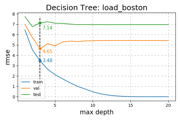
Fig. 19 RMSE of Decision Tree on the load_boston dataset varying over max depth.

Random Forest Regression

Python

model = RandomForest(objective = variance, leaf = average, max_depth = max_depth).fit(X_train, y_train)
rmse  = np.array([model.rmse(train, val, test, prune = depth) for depth in depths])

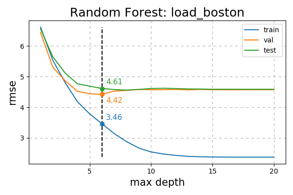
Fig. 20 RMSE of Random Forest on the load_boston dataset varying over max depth.

Classification

For the regression problem, we try out the sklearn’s load_digits dataset.

Dataset

load_digits

Optical recognition of handwritten digits dataset

Data Set Characteristics:

Number of Instances: 5620 Number of Attributes: 64 Attribute Information: 8x8 image of integer pixels in the range 0..16. Missing Attribute Values: None Creator: E. Alpaydin (alpaydin ‘@’ boun.edu.tr) Date: July; 1998

This is a copy of the test set of the UCI ML hand-written digits datasets https://archive.ics.uci.edu/ml/datasets/Optical+Recognition+of+Handwritten+Digits

The data set contains images of hand-written digits: 10 classes where each class refers to a digit.

Preprocessing programs made available by NIST were used to extract normalized bitmaps of handwritten digits from a preprinted form. From a total of 43 people, 30 contributed to the training set and different 13 to the test set. 32x32 bitmaps are divided into nonoverlapping blocks of 4x4 and the number of on pixels are counted in each block. This generates an input matrix of 8x8 where each element is an integer in the range 0..16. This reduces dimensionality and gives invariance to small distortions.

For info on NIST preprocessing routines, see M. D. Garris, J. L. Blue, G. T. Candela, D. L. Dimmick, J. Geist, P. J. Grother, S. A. Janet, and C. L. Wilson, NIST Form-Based Handprint Recognition System, NISTIR 5469, 1994.

References:

• C. Kaynak (1995) Methods of Combining Multiple Classifiers and Their Applications to Handwritten Digit Recognition, MSc Thesis, Institute of Graduate Studies in Science and Engineering, Bogazici University.

• 5. Alpaydin, C. Kaynak (1998) Cascading Classifiers, Kybernetika.

• Ken Tang and Ponnuthurai N. Suganthan and Xi Yao and A. Kai Qin. Linear dimensionalityreduction using relevance weighted LDA. School of Electrical and Electronic Engineering Nanyang Technological University. 2005.

• Claudio Gentile. A New Approximate Maximal Margin Classification Algorithm. NIPS. 2000.

Decision Tree Classification

Python

Loading the load_digits dataset

from sklearn.datasets import load_digits

X, y = load_digits(return_X_y = True)

X_train, X_val, X_test, y_train, y_val, y_test, train, val, test = train_val_test_split(X, y, random_state = 2020)

Accuracy results from fitting a Decision Tree varying over the maximum depth

# leaf function
proportion10 = proportion(10)

# Fit model once and evaluate at different depth levels
model        = DecisionTree(objective = entropy, leaf = proportion10, max_depth = max_depth).fit(X_train, y_train)
acc          = np.array([model.acc(train, val, test, prune = depth) for depth in depths])

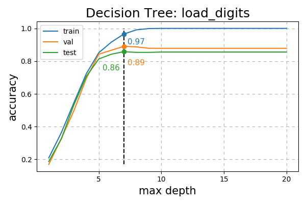
Fig. 21 Accuracy of Decision Tree on the load_digits dataset varying over max depth.

Random Forest Classification

Python

Accuracy results from fitting a Random Forest varying over the maximum depth

model = RandomForest(objective = entropy, leaf = proportion10, max_depth = max_depth).fit(X_train, y_train)
acc   = np.array([model.acc(train, val, test, prune = depth) for depth in depths])

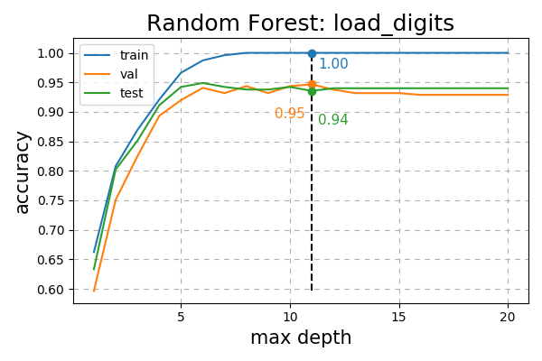
Fig. 22 Accuracy of Random Forest on the load_digits dataset varying over max depth.

References

1(1,2)

12. Breiman, Random Forests, 2001, https://link.springer.com/article/10.1023/A:1010933404324

2

20. 11. Ho, Random Decision Forests, 1995, https://ieeexplore.ieee.org/document/598994

3(1,2)

20. 11. Ho, The Random Subspace Method for Constructing Decision Forests, 1998, https://ieeexplore.ieee.org/document/709601