Value Iteration

What is Value iteration?

Value iteration is an algorithm that computes the Value function at every state assuming we have access to the mechanics behind the environment i.e. a model-based algorithm. If we have access to the environment mechanics then this is feasible, but usually we do not have access to the environment mechanics. A big assumption about the environment is it is a Markov Decision Process. If any terminology is confusing, please refer to the introduction <reinforcement-learning> to Reinforcement Learning (RL).

Markov Decision Processes

A Markov Decision Process (MDP) is a decision process that is conditioned on the most current state. Recall that the Markov property in probability has the form \(\mathbb{P}(S_{t+1}=s\mid S_1=s_1,S_2=s_2,...,S_t=s_t) = \mathbb{P}(S_{t+1}=s\mid S_t=s_t)\). Intuitively, we do not need the running history but only the most recent state as that encorporates all the information we need. This is a big assumption to make, but surprisingly a lot of environments can be thought of as an MDP e.g. chess, checkers, go etc. In more complicated state spaces this may not neccessarily be true. Lets consider a gridworld example to visualise the problem and what the solution may look like.

Example Environment - Gridworld

Consider an environment made up of identical squares forming a grid where the directions are a unit square up, right, down, and left. Suppose there is a gold terminal state which gives a \(+10\) reward for entering the state, and a bomb terminal state which gives a \(-10\) reward for entering it, and an action cost of \(-1\) whenever we take an action. We, the agent, are then interesting in finding the best path towards the gold state.

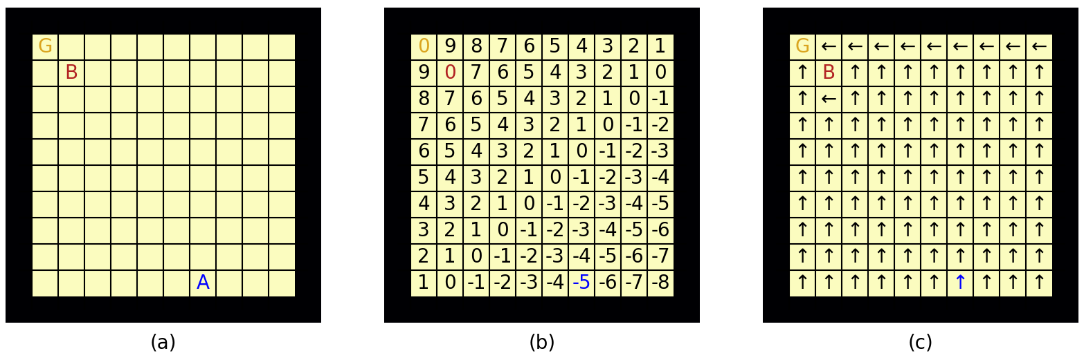
Fig. 37 (a) 2D GridWorld with a gold state in the top left, a bomb state diagonally away from the gold state and the agent on one of the bottom states. (b) Value function evaluation at every state. (c) Policy learnt by examining the immediate reward and the Value function evaluated at neighbouring states.

Lets dive into the algorithm of how to compute a Value function which has an optimal policy \(V^{\pi^{*}}(S)\) and how we can use this to compute an optimal policy \(\pi^{*}(S)\) for each \(S\in\mathcal{S}\).

Computing the Value Function and Policy

\begin{align*} \hline & \textbf{Algorithm 1} \text{ Value Iteration} \\ \hline & \textbf{Input:} \text{ State space }\mathcal{S}\text{ and positive threshold }\theta \\ & \textbf{Output: } V^{\pi^{*}}(S)\;\forall\; S\in\mathcal{S} \\ & 1. \;\; \text{Initialise } V(S) \text{ arbitrarily for all } S\in\mathcal{S} \\ & 2. \;\; \textbf{repeat} \\ & 3. \;\; \quad \Delta \leftarrow 0 \\ & 4. \;\; \quad \textbf{for } \text{each } S\in\mathcal{S} \text{ do} \\ & 5. \;\; \quad\quad v \leftarrow V(S) \\ & 6. \;\; \quad\quad V(S) \leftarrow \max_{a\in\mathcal{A}}\bigg(\mathcal{R}_S^a + \gamma \sum_{S'\in\mathcal{S}}\mathcal{P}_{SS'}^aV(S')\bigg) \\ & 7. \;\; \quad\quad \Delta \leftarrow \max (\Delta, \mid v - V(S)\mid) \\ & 8. \;\; \quad \textbf{end for} \\ & 9. \;\; \textbf{until } \Delta < \theta \\ \hline \end{align*}

Starting with the most complicated line, line 6. This line has quite a bit of notation so lets start off with the contents of the big brackets. \(\mathcal{R}_S^a\) is the expected immediate reward of taking action \(a\) when in state \(S\) and \(\mathcal{P}_{SS'}^a\) is the probability of transitioning to state \(S'\) from \(S\) by taking action \(a\). This means that \(\mathcal{R}_S^a + \gamma \sum_{S'\in\mathcal{S}}\mathcal{P}_{SS'}^aV(S')\) is a potential candidate value for \(V(S)\) as this is the recursive definition of the Value function (see here). The optimal path yields the highest Value function evaluation which justifies why we use a \(\max\) operator. \(\Delta\) is a measurement for the largest difference in Value function evaluation across the entire state space so when this becomes sufficiently small, we exit the repeating loop as the Value function has converged! Computing the policy is then done so by evaluating \(\pi(S) = \text{argmax}_{a\in\mathcal{A}} [\mathcal{R}_S^a + \gamma \sum_{S'\in\mathcal{S}}\mathcal{P}_{SS'}^a V(S')]\).

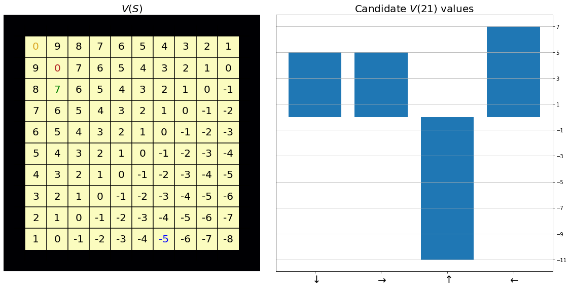
Fig. 38 On the left, we have the Value function for every state where the state of interest is highlighted in green (from the top left yellow 0, two down and one right). On the right are the candidate Value function values for the green state (21) over the action space.

It is clear that we do not want to go up into the bomb state from the above plot, and the optimal action is to go left.

Summary

Though the Value iteration algorithm is powerful, it requires a model of the environment i.e. the probabilistic state transition dynamics \(\mathcal{P}_{SS'}^a\ \forall\ S\in\mathcal{S},\ S'\in\mathcal{S},\text{ and } a\in\mathcal{A}\). In a small discrete deterministic setting, this may be possible but in large stochastic state spaces, this simply is not known and will either need to be estimated, or a method that does not rely on knowing the explicit probabilisit state transition dynamics needs to be used.