k-Means
The general clustering problem is suppose that our dataset consists purely of observations \(\mathcal{D}=\{\mathbf{x}_1,...,\mathbf{x}_n\}\) with no associated target values. The challenge is then to use the topology of \(\mathcal{D}\) to identify which observations are similar to each other, and hence, share the same associated latent target values.
The k-means algorithm is a popular simplistic algorithm that does this basing the similarity measure in \(\mathbb{L}^2\) space formally defined by [S. Lloyd, 1982] 1. The formal problem statement is; For data \(\mathcal{X} = \{\mathbf{x}_1,...,\mathbf{x}_n\} \subset \mathbb{R}^m\), a \(k\) set clustering consists of:
a partition \(\mathcal{C} = \{C_1,...,C_k\}\) of \(\mathcal{X}\) such that \(\mathcal{X} = \cup_{i=1}^k C_i\) and \(C_i \cap C_j = \emptyset\) for \(i,\ j = 1,...,k : i\neq j\)
a set \(\mathcal{Z} = \{\mathbf{z}_1,...,\mathbf{z}_k\} \subset \mathbb{R}^m\) of cluster centers
- a cost function:
- \[\begin{equation} \text{cost}(C_1,...,C_k,\mathbf{z}_1,...,\mathbf{z}_k) = \sum_{i = 1}^k \sum_{\mathbf{x}\in C_i}||\mathbf{x} - \mathbf{z}_i||_2^2, \end{equation}\]
where optimal clustering minimises the above defined cost.
Lloyd’s k-means Algorithm
k-means Example
Implementing the previously stated algorithm on a generated dataset, which clearly has four clusters and, with random initial centroid locations yields the following subplots:
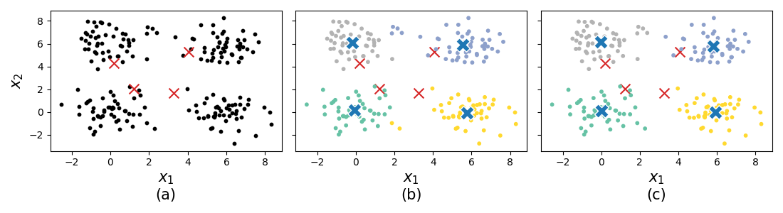
Fig. 33 (a) the simulated data with initial centroid locations. (b) the proposed new centroid locations in blue after a single iteration with convergence reached. (c) the proposed new centroid locations in blue after two iterations with convergence reached.Ӧ
How sensitive is this to the initialisation locations? Would we get similar converged locations for \(\mathbf{Z}\)? Let’s simulate the same data now changing the random seed for initialisation.
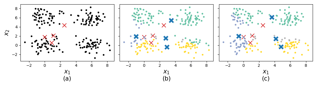
Fig. 34 (a) the simulated data with (bad) initial centroid locations. (b) the proposed new centroid locations in blue after a single iteration. (c) the proposed new centroid locations in blue after two iterations with convergence reached.
Wow - we get a converged solution that clearly is not the four clusters we were expecting! The natural question arises; How do we choose a good set of initial centroids?
It turns out the k-means++ variant from the paper [D. Arthur, 2007] 2 tackles this exact problem! The basic idea is to sample the initial centroids based on our data *sequentially* based on a probabilistic rule.
Implementation
Python
k-Means class
from   scipy.spatial.distance import cdist
import numpy as np

class KMeans():
    """
    k-Means Class

    Parameters
    ================
        k            : int
                       Number of clusters.

        initialiser  : str
                       {"uniform", "++"} denoting the initialisation.

        max_iters    : int
                       Maximum number of iterations following Lloyd's k-means algorithm.

        tol          : float
                       Minimum improvement of `cost` required (early break otherwise).

        random_state : int
                       Seed to use for np.random.seed (reproducible random results).
    """
    def __init__(self, k, initialiser = 'uniform', max_iters = 100, tol = 1e-8, random_state = None):

        initialisers = {'uniform' : self._uniform, '++' : self._plus}

        # Checks
        assert k > 0
        assert initialiser in initialisers
        assert max_iters > 0
        assert tol > 0
        assert True if random_state is None else isinstance(random_state, int)

        # Store attributes
        self.k            = k
        self.initialiser  = initialisers.get(initialiser)
        self.max_iters    = max_iters
        self.tol          = tol
        self.random_state = random_state

    @staticmethod
    def _uniform(X, k):
        """ Uniform initialisation of centroids """
        return X[np.random.choice(len(X), replace = False, size = k)]

    @staticmethod
    def _plus(X, k):
        """ ++ initialisation of centroids """
        idx = [np.random.randint(len(X))]                               # initialise the first centroid uniformly
        for i in range(1, k):
            d2 = cdist(X[idx], X, metric = 'sqeuclidean').min(axis = 0) # compute minimum distance
            p  = d2 / d2.sum()                                          # compute probability vector p
            idx.append(np.random.choice(len(X), p = p))                 # sample based on p
        return X[idx]

    def fit(self, X):
        """ Compute centroids that fit the data X. """

        np.random.seed(self.random_state)         # set seed for reproducibility

        Z  = self.Z = self.initialiser(X, self.k) # initialise centroid locations
        d2 = cdist(X, Z, metric = 'sqeuclidean')
        C  = d2.min(axis = 1).sum()               # compute total cost
        L  = self.L = [C]                         # store the "loss" (cost) over iterations
        for _ in range(self.max_iters):

            l  = d2.argmin(axis = 1)              # assign each datapoint a cluster group

            for j in range(self.k):
                Z[j] = X[l == j].mean(axis = 0)   # update the centroid locations based on a local mean

            d2 = cdist(X, Z, metric = 'sqeuclidean')
            _C = d2.min(axis = 1).sum()

            if C - _C < self.tol:                 # if improvement is not at least "tol" then early exit
                break

            C  = _C
            L.append(C)
        return self

    def predict(self, X):
        """ Assigns cluster numbers to each datapoint in `X` """
        return cdist(X, self.Z, metric = 'sqeuclidean').argmin(axis = 1)
To numerically check that the variant outperforms the vanilla algorithm, we can compute, in expectation, the converged cost.
Python
Uniform vs ++ initialisation
Uniform
L = []
for i in range(1000):
    model = KMeans(4, initialiser = '++', random_state = i)
    model.fit(X)
    L.append(model.L[-1])

print(np.mean(L))
# 436.5457007966806
++
L = []
for i in range(1000):
    model = KMeans(4, initialiser = 'uniform', random_state = i)
    model.fit(X)
    L.append(model.L[-1])

print(np.mean(L))
# 517.8733201220832
It seems like the ++ variant significantly improved the mean converged cost!
References
- 1
Lloyd, Least Squares Quantization, 1982, https://cs.nyu.edu/~roweis/csc2515-2006/readings/lloyd57.pdf
- 2
Arthur and S. Vassilvitskii, k-Means++: The Advantages of Careful Seeding, 2007, https://theory.stanford.edu/~sergei/papers/kMeansPP-soda.pdf