Linear Regression
From the theory of general regression, we assume the our functional map \(f\) is a linear line. The below illustrates a one dimensional dataset as the black scatter points and we are interested in learning the equation of the red line.
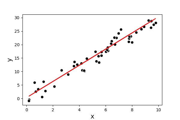
Fig. 1 Example simulated data for linear regression.
The above one-dimensional \(\mathbf{X}\in\mathbb{R}^{n,1}\) is easy for us to visualise and we can guess that line by visual inspection. What happens if \(\mathbf{X}\in\mathbb{R}^{n,m}\) and \(m\) is much larger than \(1\)? We simply cannot visualise all of it at the same time anymore, and so, require a more robust method of finding the best straight line that fits our dataset.
Ordinary Least Squares
The method of Ordinary Least Squares (OLS) is the most popular way to help compute our line but before delving into that, we need to define a few terms:
model estimate: \(\mathbf{\hat{y}} = \mathbf{Xw} + b\)
model parameters: the weight vector \(\mathbf{w}\) and bias / intercept \(b\)
Now let us assume that the dataset \(\mathcal{D}\) was generated through a similar process whereby the \(i\)-th instance of our dataset is defined by \(y_i = \mathbf{x}_i^\text{T}\mathbf{w} + b + \epsilon\) where \(\epsilon\overset{iid}{\sim}\mathcal{N}(0,\sigma^2)\) for some unknown \(\sigma^2\). This random pertubation term \(\epsilon\) may be due to slight mis-measurements of the target variable, or we do not have the complete set of measurements and have only the \(m\) set of measurements etc. From this, we can say that \(y_i\mid\mathbf{x}_i, \mathbf{w}, b, \sigma^2 \overset{iid}{\sim}\mathcal{N}(\mathbf{x}_i^\text{T}\mathbf{w} + b,\sigma^2)\), which for the entire dataset would be \(\mathbf{y}\mid\mathbf{X},\mathbf{w}, b, \sigma^2\sim\mathcal{N}(\mathbf{Xw} + b, \sigma^2\mathbf{I})\) where \(\mathbf{I}\) is the identity matrix. The logpdf of this Normal distribution is then:
We wish to maximise the log probability which is the same is maximising the last term which can be re-written as a vector norm,
where \(\mid\mid \mathbf{z}\mid\mid_p^q\ := \left(\sum_{i=1}^n \mid z\ \mid ^p\right)^{q/p}\) with the setting \(p=q=2\) resulting in the total squared residual error. Dividing by \(n\) yields the popular metric Mean Squared Error (MSE) which does not change the optimal \(\mathbf{w}\) and \(b\) parameters. By tweaking the notation a bit, we can make the problem appear easier. Let us denote \(\mathbf{\tilde{X}} = [\mathbf{1},\mathbf{X}]\) and \(\mathbf{\tilde{w}} = [b,\mathbf{w}^{\text{T}}]^{\text{T}}\), then we are interested in minimising
At this point we will omit the tilde symbol for notational convenience and set \(\mathcal{L}\) to be the loss function defined by the term to be minimised above. By considering vector calculus we have:
So from the above, \(\mathbf{\hat{w}}\) is obtained by solving the final linear system we arrived at assuming the inverse of \(\mathbf{X}^\text{T}\mathbf{X}\) exists. To prove that this solution is indeed a minimising solution rather than a maximising one, we can differentiate again to find the second derivative is \(\mathbf{X}^\text{T}\mathbf{X}\), for which if the inverse exists, \(\mathbf{X}^\text{T}\mathbf{X}\) is symmetric semi-positive definite.
Example: UCI Wine Data Set
In this example we will use data from the UCI repository: Wine Dataset.
Dataset
UCI: Wine Quality Dataset
Source:
Paulo Cortez, University of Minho, Guimarães, Portugal, http://www3.dsi.uminho.pt/pcortez A. Cerdeira, F. Almeida, T. Matos and J. Reis, Viticulture Commission of the Vinho Verde Region(CVRVV), Porto, Portugal @2009
Data Set Information:
The two datasets are related to red and white variants of the Portuguese “Vinho Verde” wine. For more details, consult: [Web Link 1] or the reference [Cortez et al., 2009]. Due to privacy and logistic issues, only physicochemical (inputs) and sensory (the output) variables are available (e.g. there is no data about grape types, wine brand, wine selling price, etc.).
These datasets can be viewed as classification or regression tasks. The classes are ordered and not balanced (e.g. there are many more normal wines than excellent or poor ones). Outlier detection algorithms could be used to detect the few excellent or poor wines. Also, we are not sure if all input variables are relevant. So it could be interesting to test feature selection methods.
Attribute Information:
For more information, read [Cortez et al., 2009].
Input variables (based on physicochemical tests):
fixed acidity
volatile acidity
citric acid
residual sugar
chlorides
free sulfur dioxide
total sulfur dioxide
density
pH
sulphates
alcohol
Output variable (based on sensory data):
quality (score between 0 and 10)
Relevant Papers:
P. Cortez, A. Cerdeira, F. Almeida, T. Matos and J. Reis. Modeling wine preferences by data mining from physicochemical properties. In Decision Support Systems, Elsevier, 47(4):547-553, 2009.
Available at: [Web Link 2]
Before we go into the model fitting, lets explore the linear relationship between our observed and target variables.
Python
Load and visualise the data
from   sklearn.model_selection import train_test_split
from   matplotlib              import pyplot as plt

import seaborn as sns
import pandas  as pd
import numpy   as np

data_r = pd.read_csv('data/winequality-red.csv', sep = ';')
data_w = pd.read_csv('data/winequality-white.csv', sep = ';')

# Show numbers with 2 decimal places, remove colour bar, set the min and max numbers (for colouring purposes) as -1, and 1
sns.heatmap(data_r.corr(), annot = True, fmt = '.2f', cbar = False, vmin = -1, vmax = 1, cmap = 'RdBu')
plt.show()
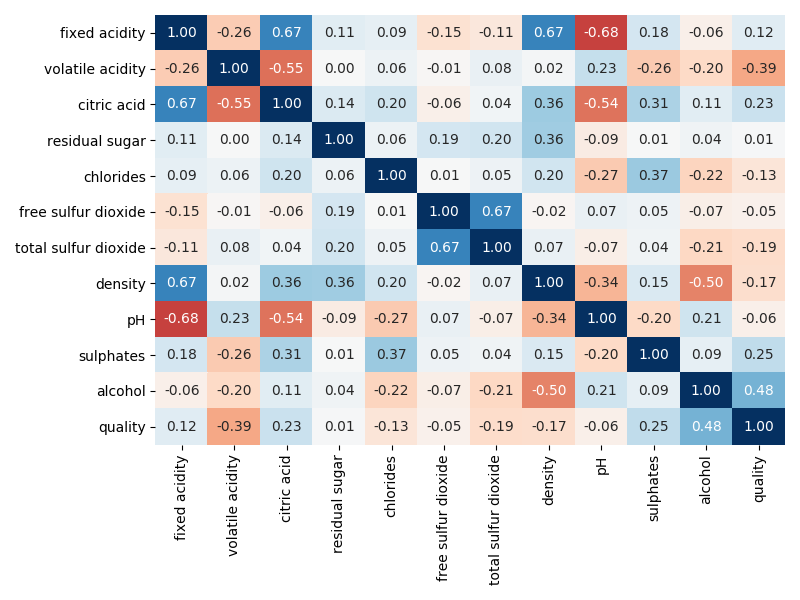
Fig. 2 Correlation heatmap for the wine dataset.
From the above, we see that the target variable is wine quality with the rest being measurements that construct the columns of \(\mathbf{X}\). From the last row, we expect the most important variables to be alcohol and volatile acidity whilst the least important to be residual sugar. These numbers are a measure of the linear relationship between each pair of variables with -1 meaning a perfect negative linear relationship and +1 a perfect positive linear relationship. If we want more detail behind these numbers we would then look at the pairplot between all variables but generally that is a huge mess with no real gains especially when \(m\) is a large number.
Python
Define a few helper functions to get us started
def get_data(df, test_size = 0.2, random_state = None):
    """ Given a pandas.DataFrame object, splits into X and y arrays then returns X_train, X_test, y_train, y_test """
    X, y = df.iloc[:,:-1].values, df.iloc[:,[-1]].values # Assumes df = [X, y] (y is the final column)
    return train_test_split(X, y, test_size = test_size, random_state = random_state)

def compute_params(X, y):
    """ Computes analytical solution returning b, W """
    X  = np.insert(X, 0, 1, 1)
    bw =  np.linalg.solve(X.T @ X, X.T @ y)
    return bw[0], bw[1:] # b, w

def predict(X, w, b):
    """ Computes y_pred """
    return X @ w + b

def rmse(y_true, y_pred):
    """ computes the rmse between y_true and y_pred """
    return np.sqrt(np.mean(np.square(y_true - y_pred)))
Python
Execution of previous code to dataset
# Red Wine
X_train, X_test, y_train, y_test = get_data(data_r, random_state = 2020)

b, w        = compute_params(X_train, y_train)
y_train_hat = predict(X_train, w, b)
y_test_hat  = predict(X_test , w, b)

print(rmse(y_train, y_train_hat), rmse(y_test, y_test_hat))
# (0.6473446749592081, 0.6396080364793854)

# White Wine
X_train, X_test, y_train, y_test = get_data(data_w, random_state = 2020)

b, w        = compute_params(X_train, y_train)
y_train_hat = predict(X_train, w, b)
y_test_hat  = predict(X_test , w, b)

print(rmse(y_train, y_train_hat), rmse(y_test, y_test_hat))
# (0.7527038586550729, 0.7431843663321125)
The above results show that the training root mean squared error metric is similar for both the train and test datasets which means our model has neither overfitted nor underfitted. We can examine the weights to check if our previous hypothesis that alcohol and volatile acidity were important.
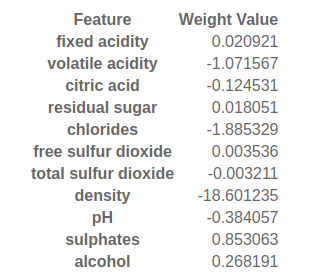
Fig. 3 Weights of linear model fitted to the wine dataset.
We unexpectedly have as the most important feature, density with a weight value of -18.6 which does not agree with our heatmap earier. This is because each feature has a different scale. Consider an example of computing the perimeter of a rectangle given the features height and width. If one were measured in cm and the other in mm the weights would have to be 2 and 200 as the scales are different. What we can do in our case here is to standardise it assuming that each feature follows a univariate Normal. In plain English, for each column, subtract the mean and divide by the standard deviation FROM THE TRAIN SET!
Lets tidy up the code into a class and implement the standardising transformation first.
Python
Linear Regression class
1 2 3 4 5 6 7 8 9 10 11 12 13 14 15 16 17 18 19 20 21 22 23 24 25 26 27 28 29 30 31 | class LinearRegression():
"""
Linear Regression Class
Parameters
==========
standardise : bool
If True, transforms X -> Z based on the X values used in the fit call, otherwise, X -> X.
"""
mu = 0
sigma = 1
def __init__(self, standardise = False):
self.standardise = standardise
def __transform(self, X):
Z = (X - self.mu) / self.sigma
return Z
def fit(self, X, y):
if self.standardise:
self.mu, self.sigma = X.mean(axis = 0, keepdims = True), X.std(axis = 0, keepdims = True)
X = self.__transform(X)
X = np.insert(X, 0 , 1, 1)
bw = np.linalg.solve(X.T @ X, X.T @ y)
self.b = bw[0]
self.w = bw[1:]
return self
def __call__(self, X):
return self.__transform(X) @ self.w + self.b
|
Python
Getting the weight attribute from our Linear Regression class
model = LinearRegression(standardise = True).fit(X_train, y_train)

# print(model.w)
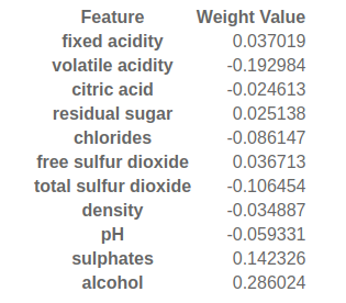
Fig. 4 Weights of a linear model fitted to the standardised wine dataset.
The above agrees with our hypothesis that the most important features are alcohol and volatile acidity whilst the least important is residual sugar!